# load packages
library(tidyverse)        # for data wrangling
library(broom)            # for formatting regression output
library(fivethirtyeight)  # for the fandango dataset
library(knitr)            # for formatting tables
library(patchwork)        # for arranging graphs

# set default theme and larger font size for ggplot2
ggplot2::theme_set(ggplot2::theme_bw(base_size = 16))

# set default figure parameters for knitr
knitr::opts_chunk$set(
  fig.width = 8,
  fig.asp = 0.618,
  fig.retina = 3,
  dpi = 300,
  out.width = "80%"
)Simple linear regression
Jan 14, 2025
Source: R for Data Science with additions from The Art of Statistics: How to Learn from Data.
Source:R for Data Science
Movie scores
- Data behind the FiveThirtyEight story Be Suspicious Of Online Movie Ratings, Especially Fandango’s
- In the fivethirtyeight package:
fandango - Contains every film released in 2014 and 2015 that has at least 30 fan reviews on Fandango, an IMDb score, Rotten Tomatoes critic and user ratings, and Metacritic critic and user scores


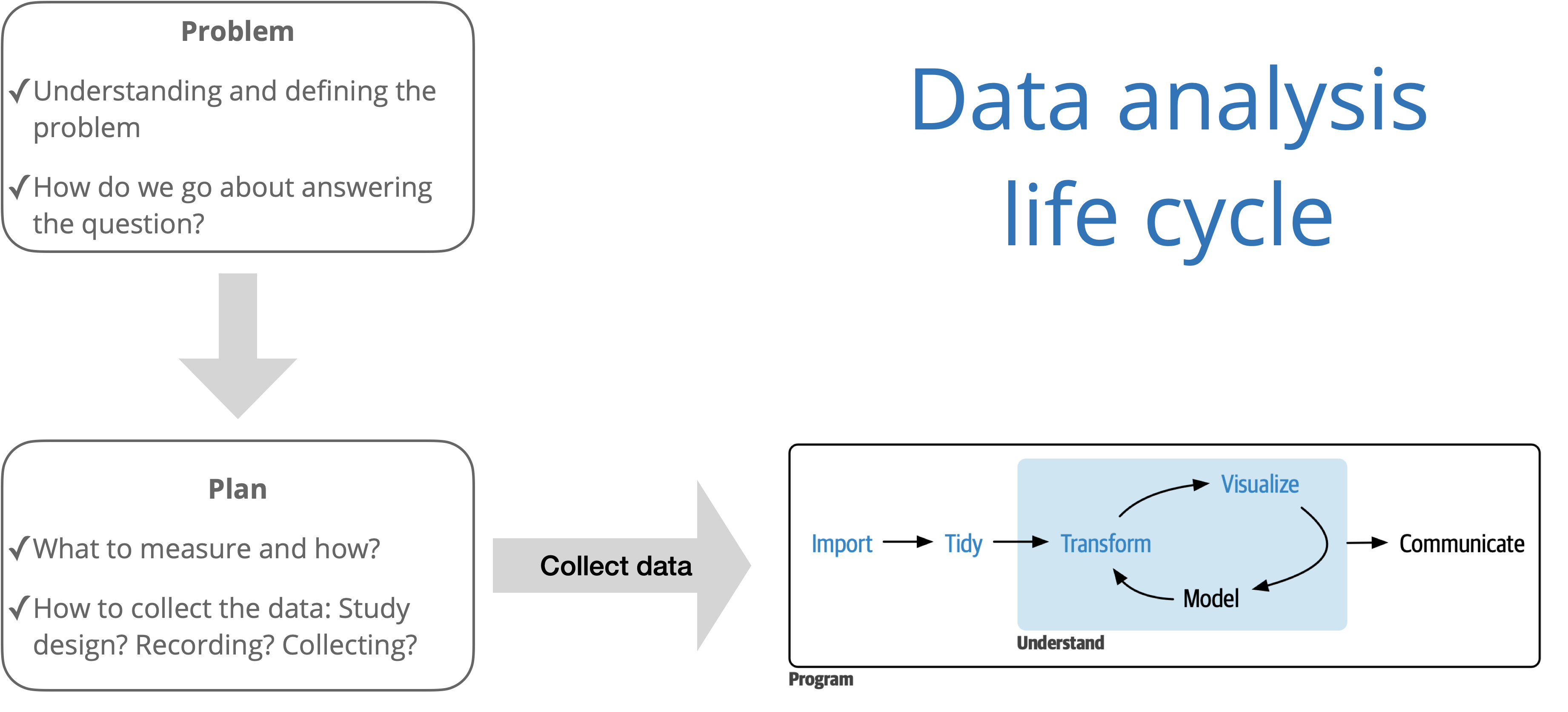
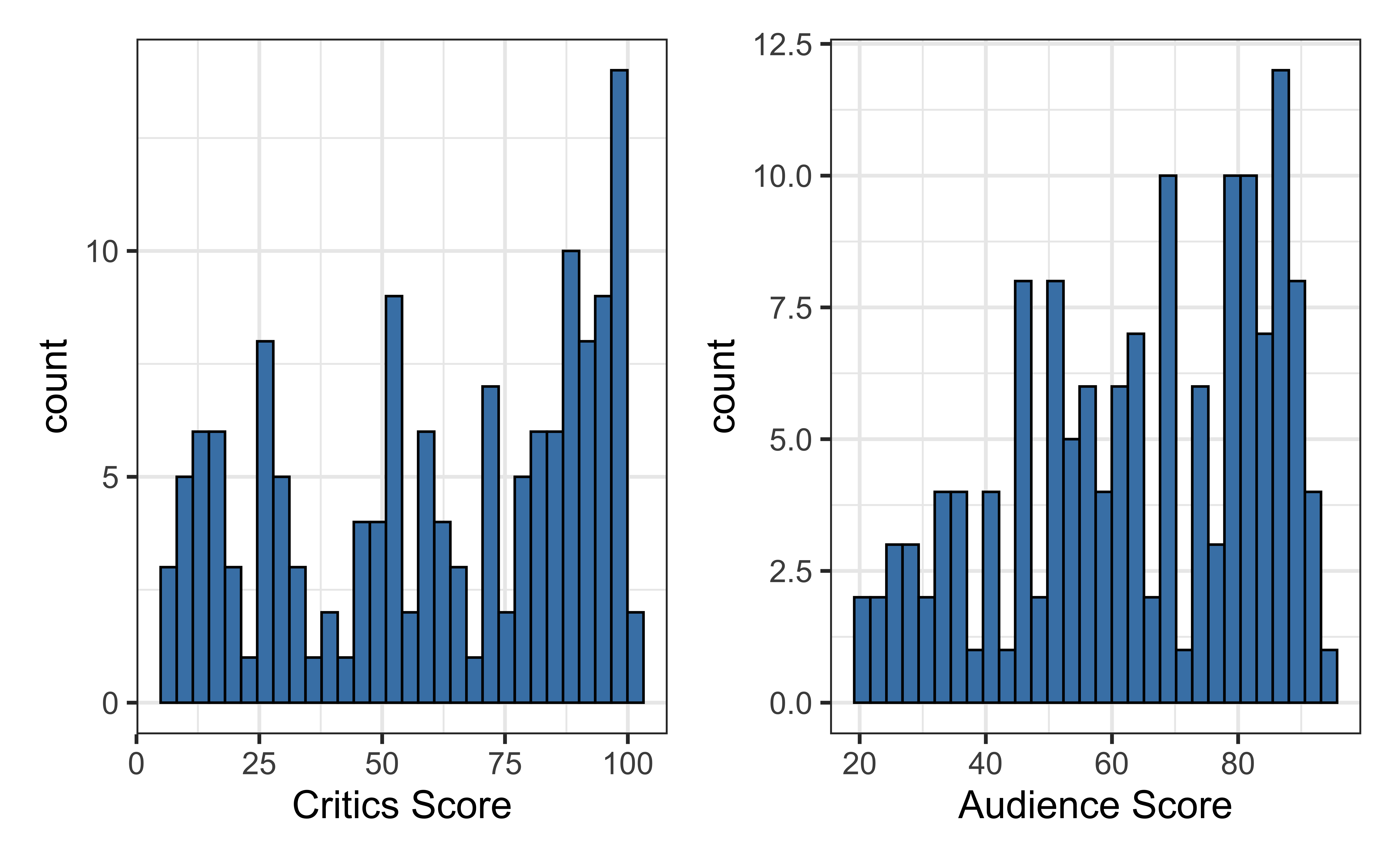
Univariate exploratory data analysis (EDA)
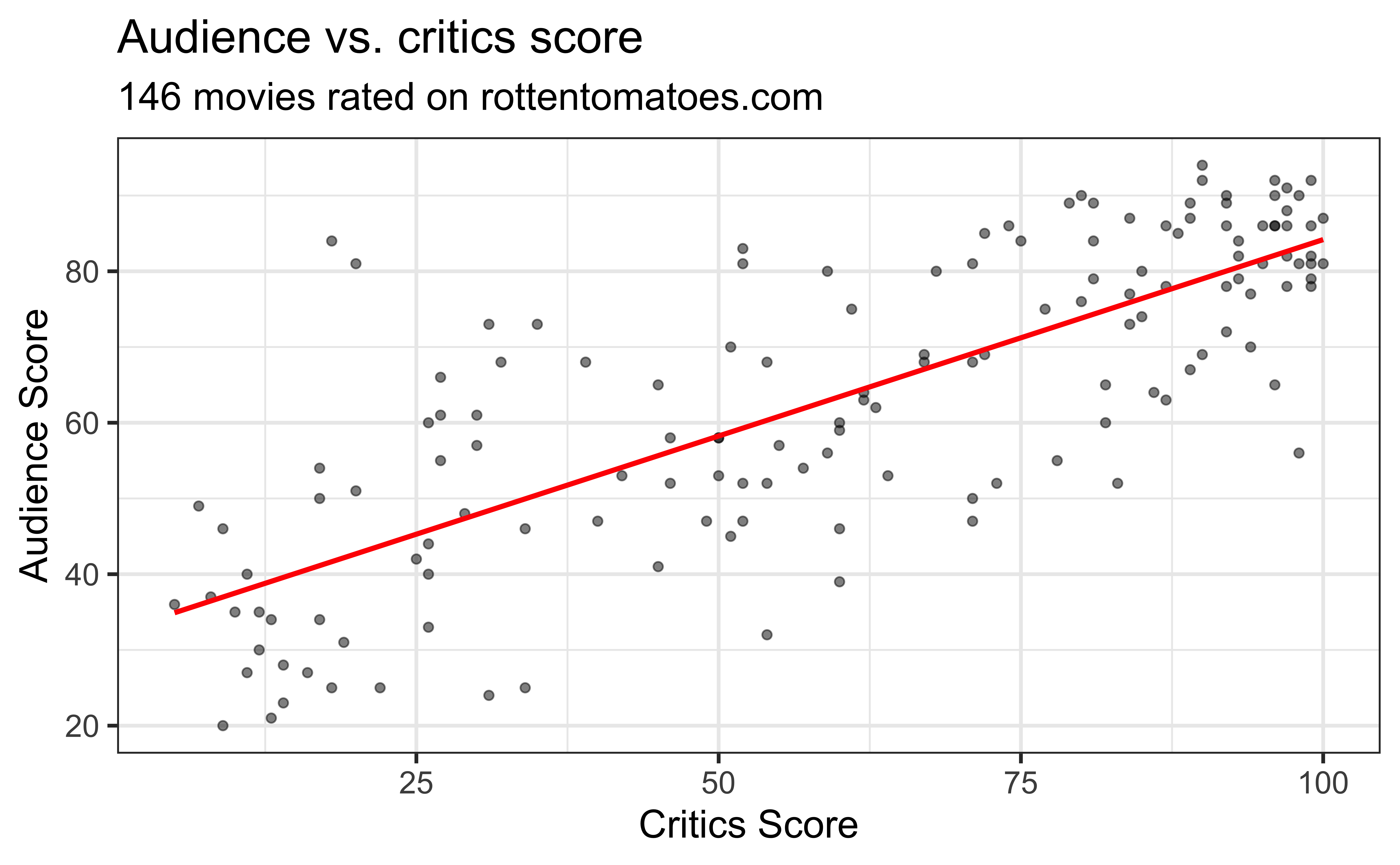
The data set contains the “Tomatometer” score (critics) and audience score (audience) for 146 movies rated on rottentomatoes.com.
Bivariate EDA
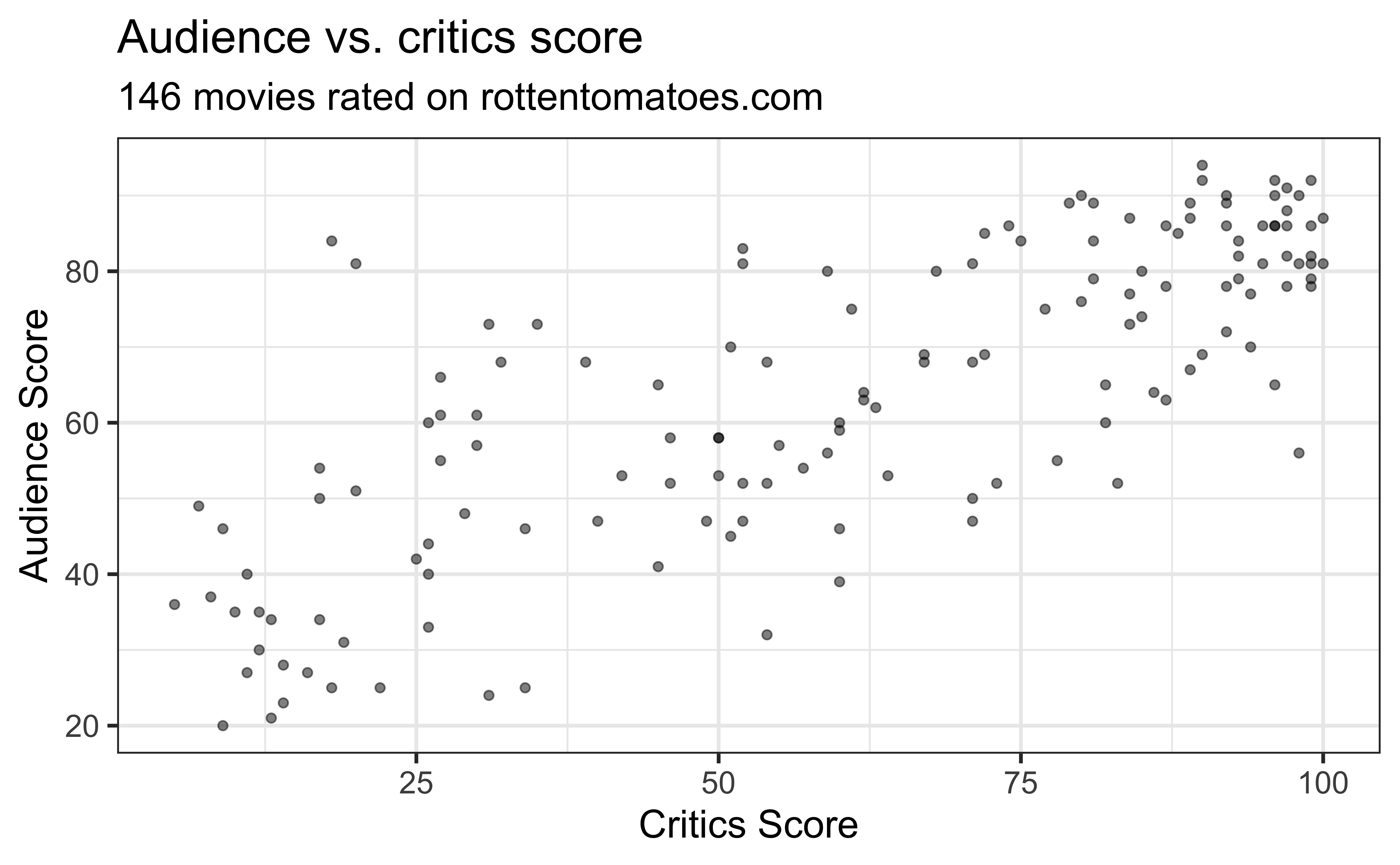
Bivariate EDA
Goal: Fit a line to describe the relationship between the critics score and audience score.
Terminology
Response, \(Y\): variable describing the outcome of interest
Predictor, \(X\): variable we use to help understand the variability in the response

Regression model
\[\begin{aligned} Y &= \color{purple}{\textbf{Model}} + \color{black}\text{Error} \\[8pt]
&= \color{purple}{f(X)} + \color{black}\epsilon \\[8pt]
&= \color{purple}{E(Y|X)} + \color{black}\epsilon \\[8pt]
&= \color{purple}{\mu_{Y|X}} + \color{black}\epsilon \end{aligned}\]
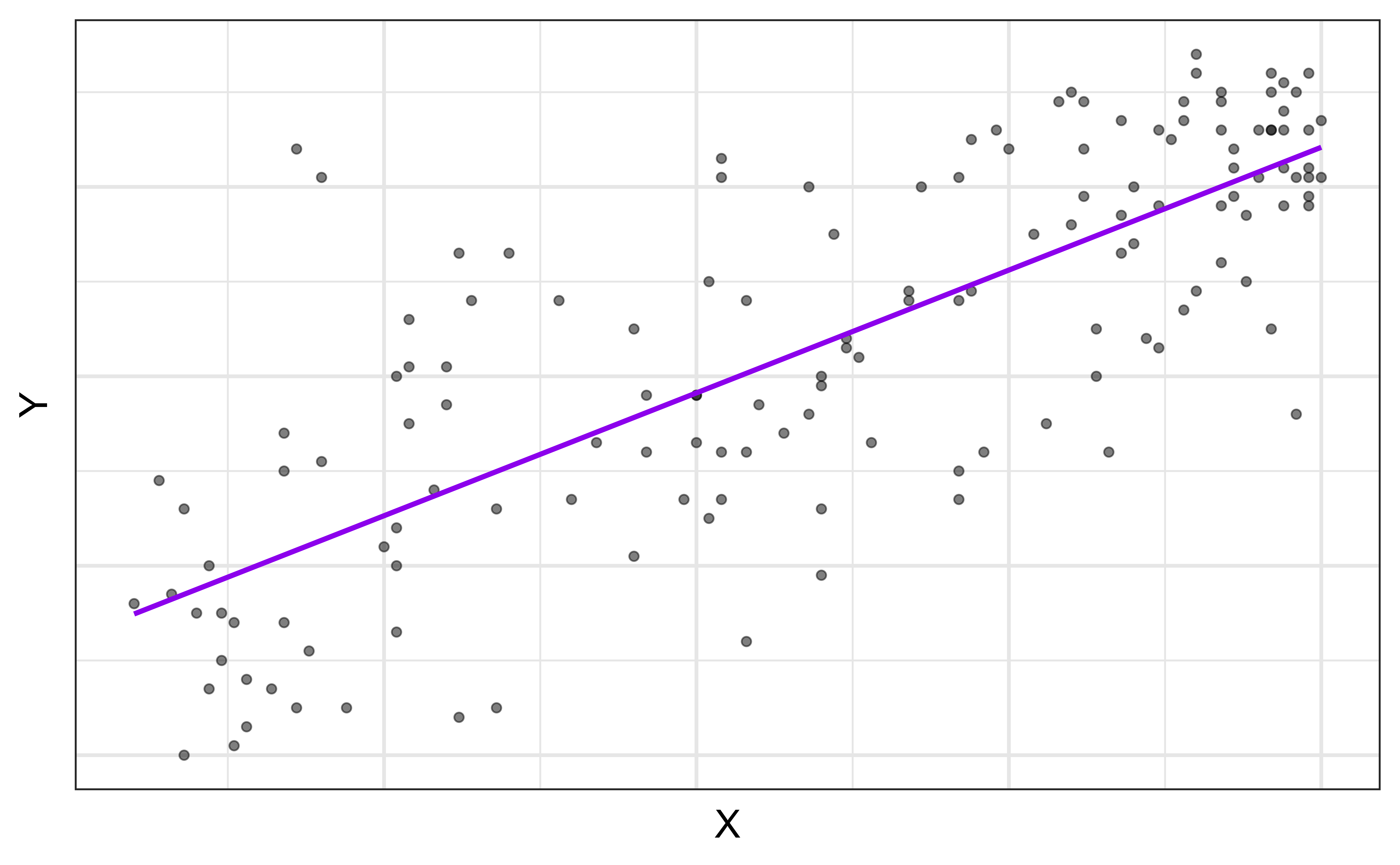
\(E(Y|X) = \mu_{Y|X}\), the mean value of \(Y\) given a particular value of \(X\).
Regression model
\[ \begin{aligned} Y &= \color{purple}{\textbf{Model}} + \color{blue}{\textbf{Error}} \\[8pt] &= \color{purple}{f(X)} + \color{blue}{\epsilon}\\[8pt] &= \color{purple}{E(Y|X)} + \color{blue}{\epsilon}\\[8pt] &= \color{purple}{\mu_{Y|X}} + \color{blue}{\epsilon} \\ \end{aligned} \]
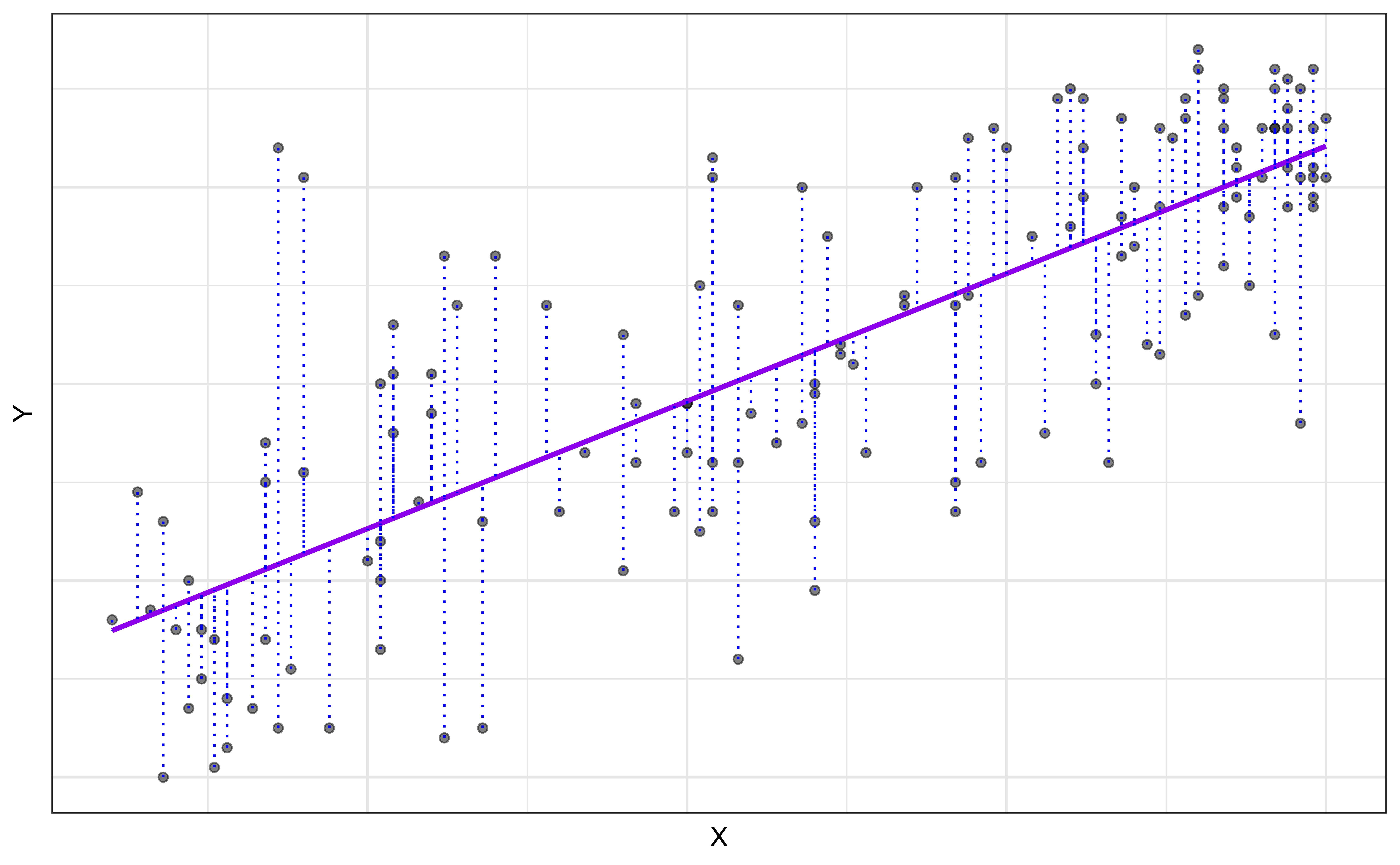
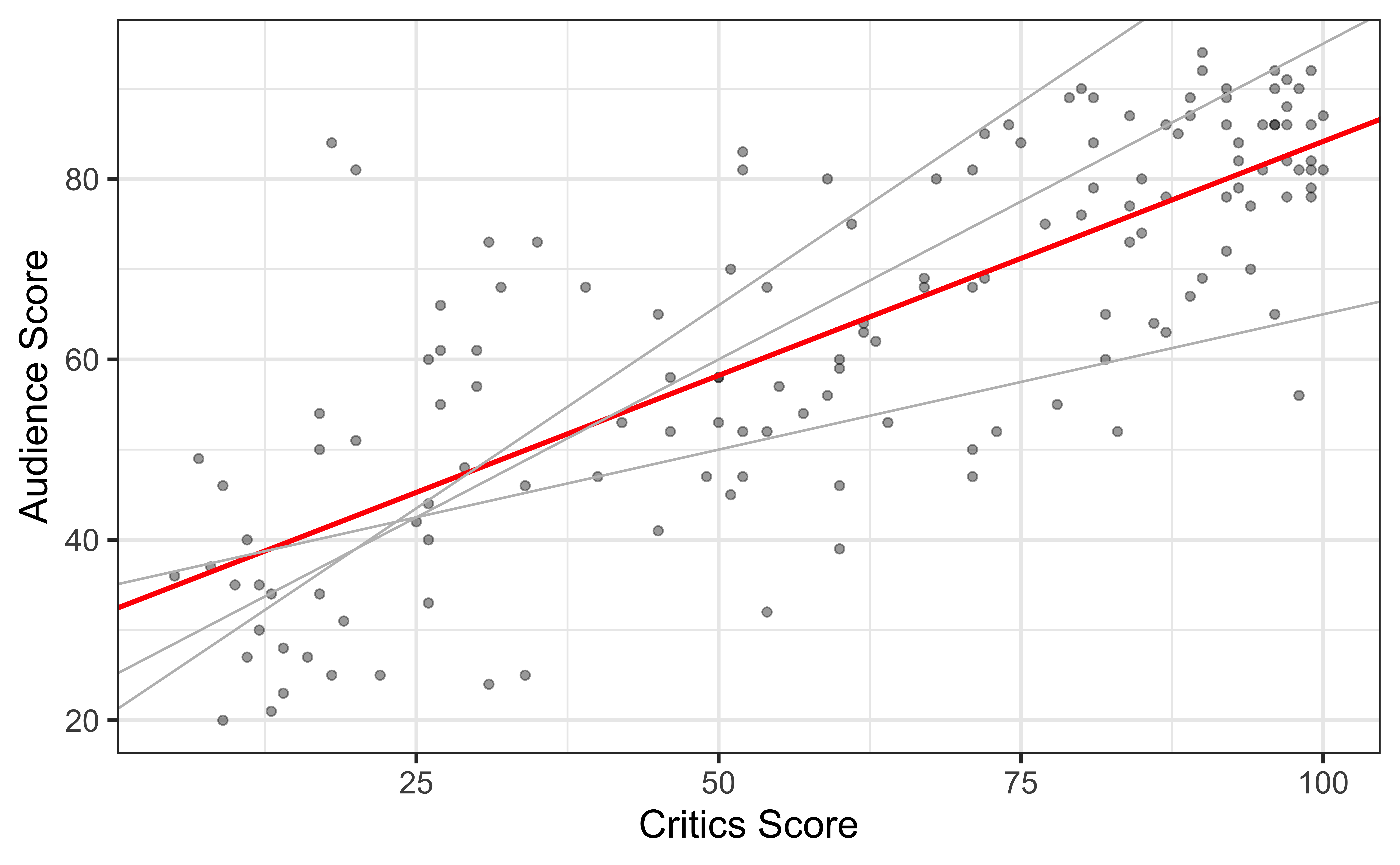
Estimating \(\hat{\beta}_1\) and \(\hat{\beta}_0\)
Residuals
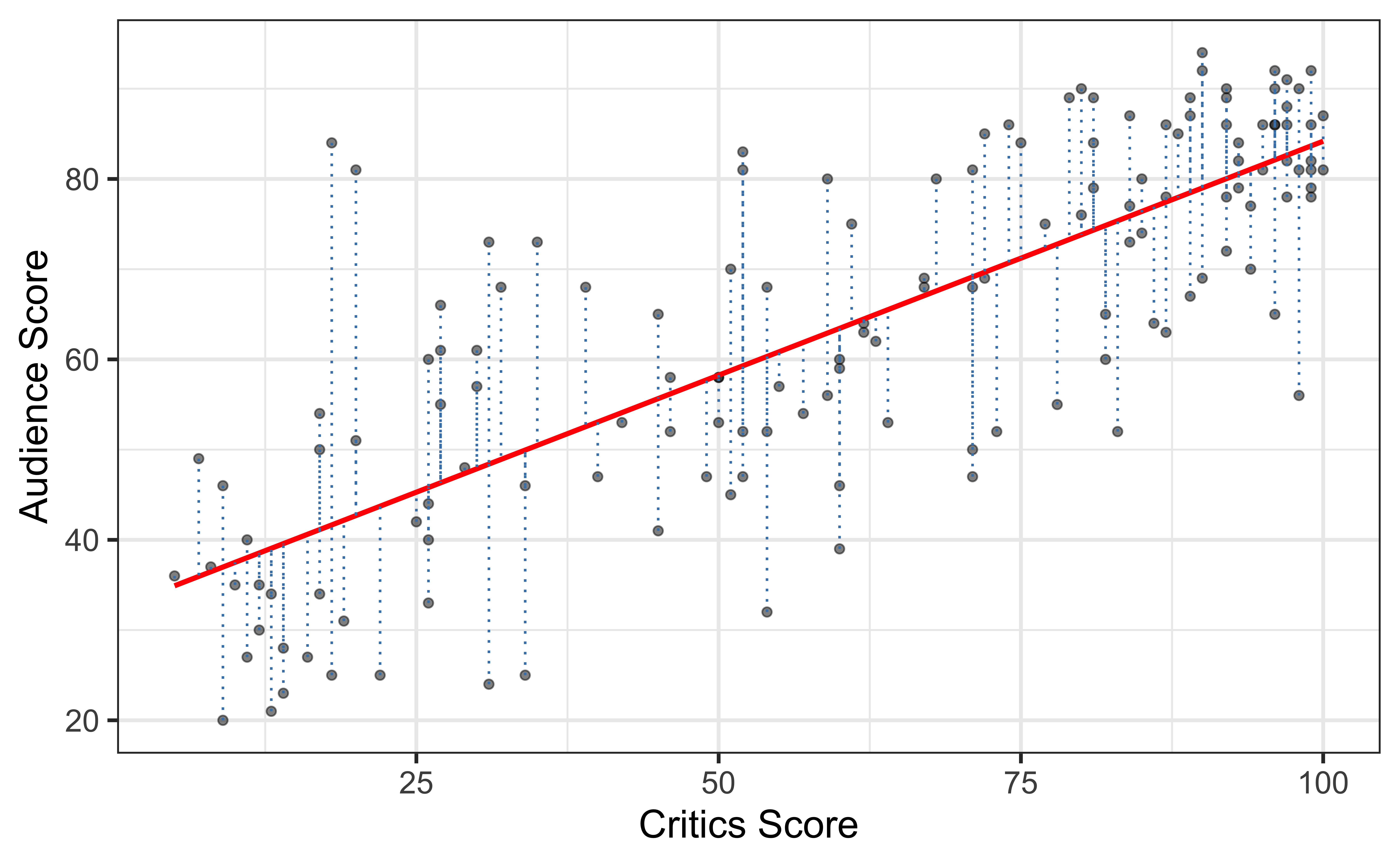
\[\text{residual} = \text{observed} - \text{predicted} = y_i - \hat{y}_i\]