Inference for regression
Cont’d
Feb 06, 2025
Announcements
HW 02 due Thursday, February 13 at 11:59pm
- Released after class
Lecture recordings available until start of exam, February 18 at 10:05am
- See link under “Exam 01” on menu of course website
Statistics experience due Tuesday, April 22
Topics
Understand statistical inference in the context of regression
Describe the assumptions for regression
Understand connection between distribution of residuals and inferential procedures
Conduct inference on a single coefficient
Computing setup
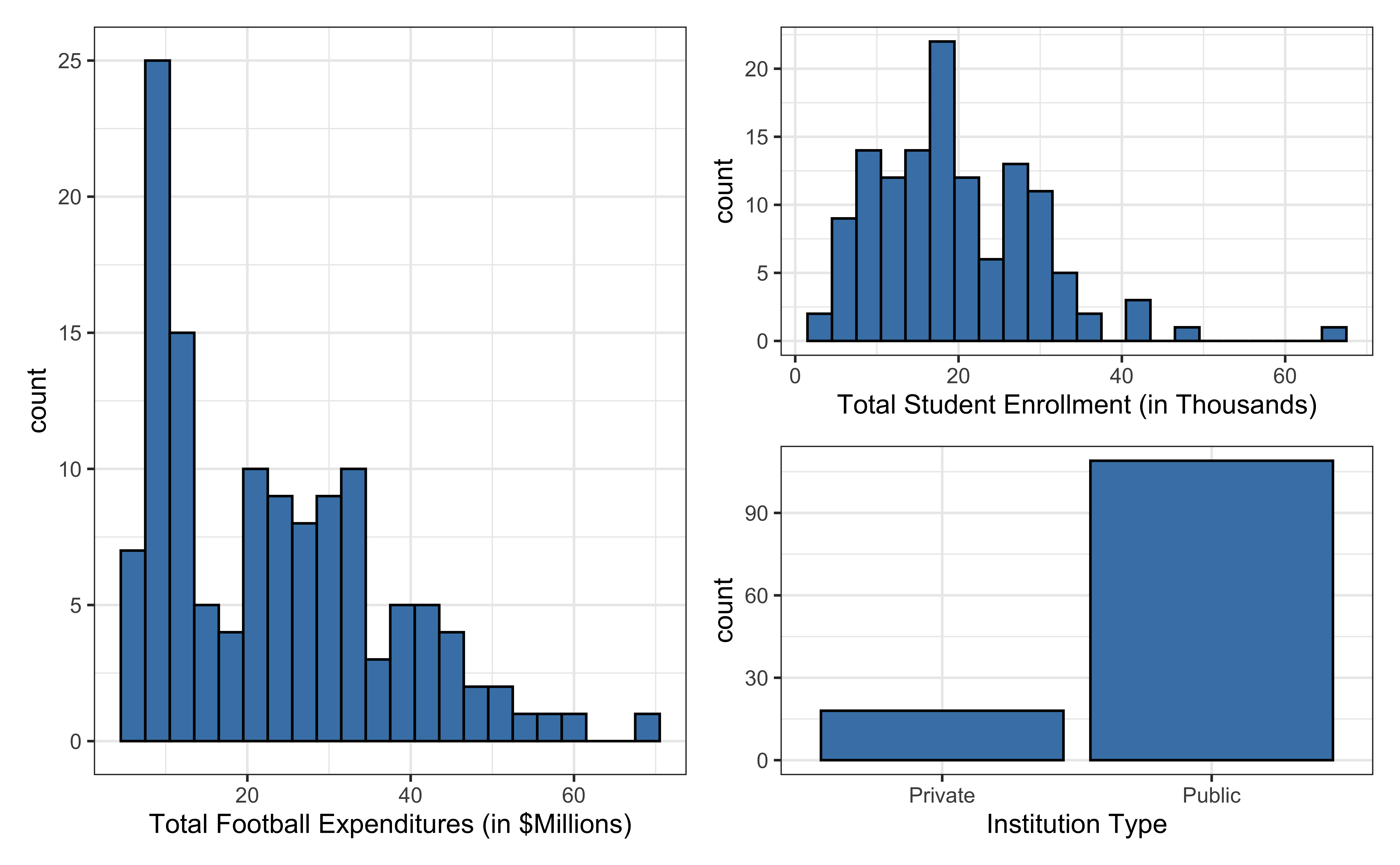
Data: NCAA Football expenditures
Today’s data come from Equity in Athletics Data Analysis and includes information about sports expenditures and revenues for colleges and universities in the United States. This data set was featured in a March 2022 Tidy Tuesday.
We will focus on the 2019 - 2020 season expenditures on football for institutions in the NCAA - Division 1 FBS. The variables are :
total_exp_m: Total expenditures on football in the 2019 - 2020 academic year (in millions USD)enrollment_th: Total student enrollment in the 2019 - 2020 academic year (in thousands)type: institution type (Public or Private)
Univariate EDA
Bivariate EDA
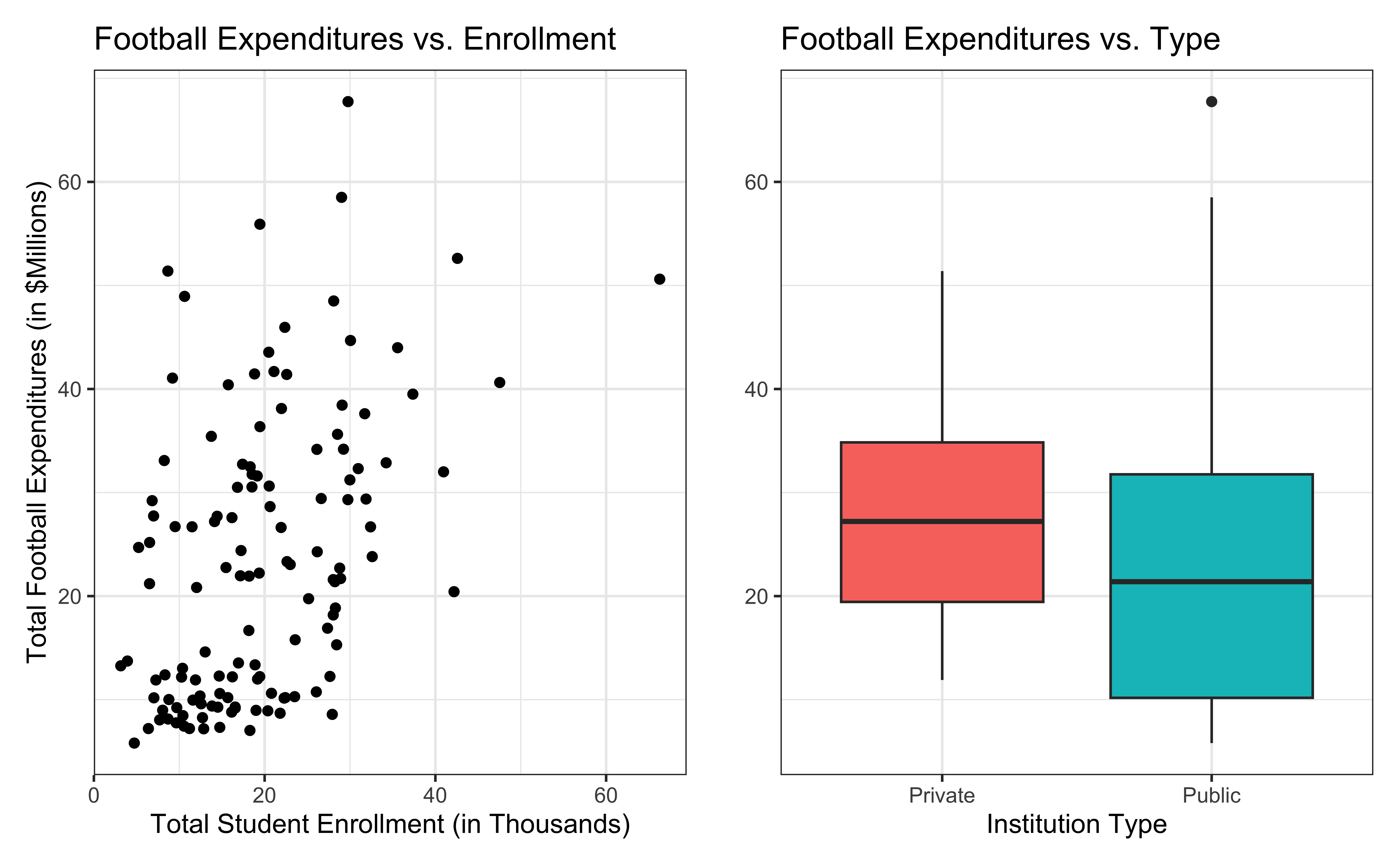
Regression model
exp_fit <- lm(total_exp_m ~ enrollment_th + type, data = football)
tidy(exp_fit) |>
kable(digits = 3)| term | estimate | std.error | statistic | p.value |
|---|---|---|---|---|
| (Intercept) | 19.332 | 2.984 | 6.478 | 0 |
| enrollment_th | 0.780 | 0.110 | 7.074 | 0 |
| typePublic | -13.226 | 3.153 | -4.195 | 0 |
For every additional 1,000 students, we expect an institution’s total expenditures on football to increase by $780,000, on average, holding institution type constant.
From sample to population
For every additional 1,000 students, we expect an institution’s total expenditures on football to increase by $780,000, on average, holding institution type constant.
- This estimate is valid for the single sample of 127 higher education institutions in the 2019 - 2020 academic year.
- But what if we’re not interested quantifying the relationship between student enrollment, institution type, and football expenditures for this single sample?
- What if we want to say something about the relationship between these variables for all colleges and universities with football programs and across different years?
Inference for regression
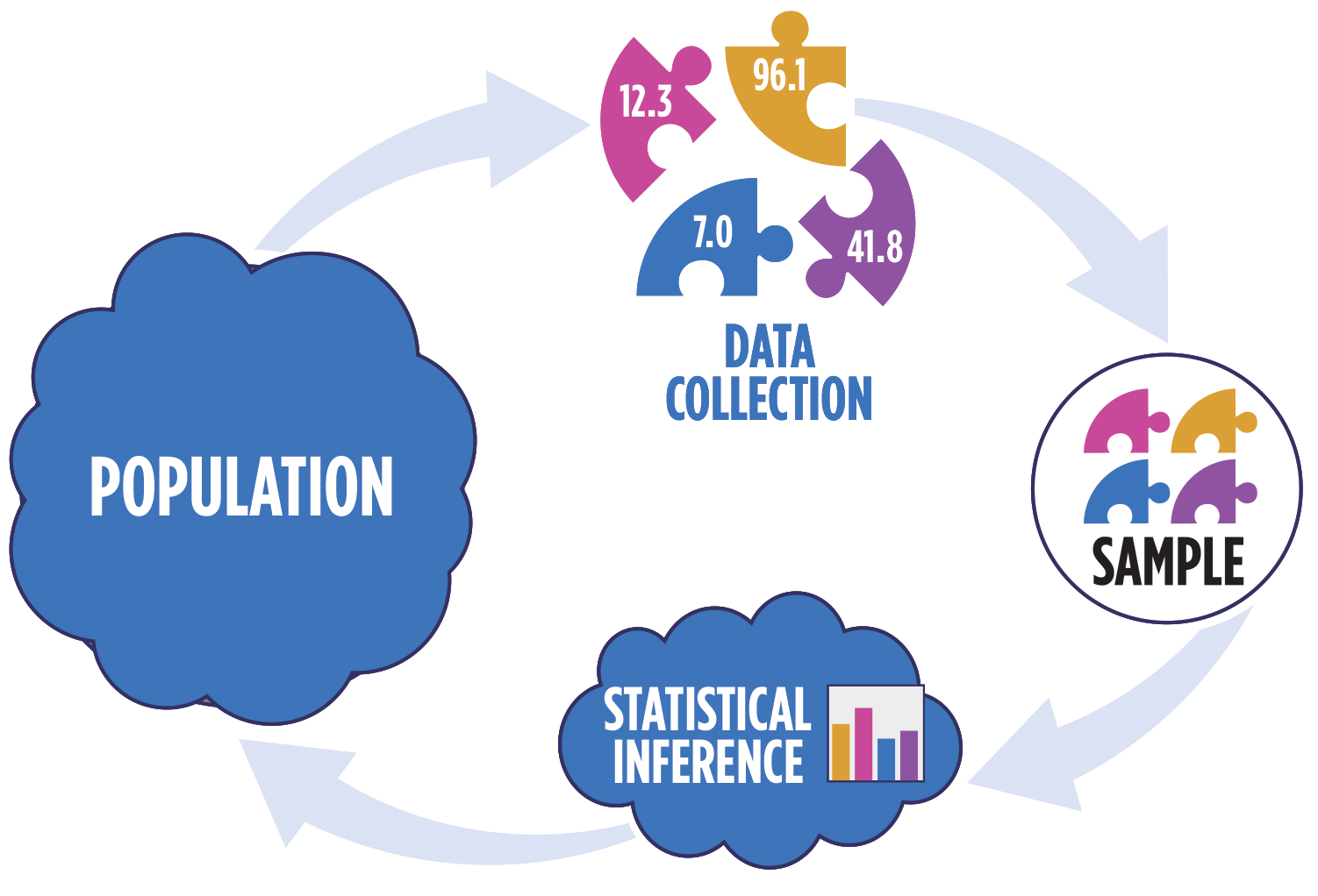
Statistical inference
Statistical inference provides methods and tools so we can use the single observed sample to make valid statements (inferences) about the population it comes from
For our inferences to be valid, the sample should be representative (ideally random) of the population we’re interested in
Linear regression model
\[\begin{aligned} \mathbf{Y} = \mathbf{X}\boldsymbol{\beta} + \boldsymbol{\epsilon}, \hspace{8mm} \boldsymbol{\epsilon} \sim N(\mathbf{0}, \sigma^2_{\epsilon}\mathbf{I}) \end{aligned} \]
such that the errors are independent and normally distributed.
- Independent: Knowing the error term for one observation doesn’t tell us about the error term for another observation
- Normally distributed: The distribution follows a particular mathematical model that is unimodal and symmetric
Visualizing distribution of \(\mathbf{y}|\mathbf{X}\)
\[ \mathbf{y}|\mathbf{X} \sim N(\mathbf{X}\boldsymbol{\beta}, \sigma_\epsilon^2\mathbf{I}) \]
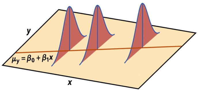
Image source: Introduction to the Practice of Statistics (5th ed)
Linear transformation of normal random variable
Suppose \(\mathbf{z}\) is a (multivariate) normal random variable such that \(\mathbf{z} \sim N(\boldsymbol{\mu}, \boldsymbol{\Sigma})\), \(\mathbf{A}\) is a matrix of constants, and \(\mathbf{b}\) is a vector of constants.
A linear transformation of \(\mathbf{z}\) is also multivariate normal, such that
\[ \mathbf{A}\mathbf{z} + \mathbf{b} \sim N(\mathbf{A}\boldsymbol{\mu} + \mathbf{b}, \mathbf{A}\boldsymbol{\Sigma}\mathbf{A}^\mathsf{T}) \]
Explain why \(\mathbf{y}|\mathbf{X}\) is normally distributed.
Assumptions for regression
\[ \mathbf{y}|\mathbf{X} \sim N(\mathbf{X}\boldsymbol{\beta}, \sigma_\epsilon^2\mathbf{I}) \]
- Linearity: There is a linear relationship between the response and predictor variables.
- Constant Variance: The variability about the least squares line is generally constant.
- Normality: The distribution of the residuals is approximately normal.
- Independence: The residuals are independent from one another.
Estimating \(\sigma^2_{\epsilon}\)
Once we fit the model, we can use the residuals to estimate \(\sigma_{\epsilon}^2\)
The estimated value \(\hat{\sigma}^2_{\epsilon}\) is needed for hypothesis testing and constructing confidence intervals for regression
\[ \hat{\sigma}^2_\epsilon = \frac{SSR}{n - p - 1} = \frac{\mathbf{e}^\mathsf{T}\mathbf{e}}{n-p-1} \]
- The regression standard error \(\hat{\sigma}_{\epsilon}\) is a measure of the average distance between the observations and regression line
\[ \hat{\sigma}_\epsilon = \sqrt{\frac{SSR}{n - p - 1}} = \hat{\sigma}_\epsilon = \sqrt{\frac{\mathbf{e}^\mathsf{T}\mathbf{e}}{n - p - 1}} \]
Inference for a single coefficient
Inference for \(\beta_j\)
We often want to conduct inference on individual model coefficients
Hypothesis test: Is there a linear relationship between the response and \(x_j\)?
Confidence interval: What is a plausible range of values \(\beta_j\) can take?
But first we need to understand the distribution of \(\hat{\beta}_j\)
Sampling distribution of \(\hat{\beta}\)
A sampling distribution is the probability distribution of a statistic for a large number of random samples of size \(n\) from a population
The sampling distribution of \(\hat{\boldsymbol{\beta}}\) is the probability distribution of the estimated coefficients if we repeatedly took samples of size \(n\) and fit the regression model
\[ \hat{\boldsymbol{\beta}} \sim N(\boldsymbol{\beta}, \sigma^2_\epsilon(\mathbf{X}^\mathsf{T}\mathbf{X})^{-1}) \]
The estimated coefficients \(\hat{\boldsymbol{\beta}}\) are normally distributed with
\[ E(\hat{\boldsymbol{\beta}}) = \boldsymbol{\beta} \hspace{10mm} Var(\hat{\boldsymbol{\beta}}) = \sigma^2_{\epsilon}(\boldsymbol{X}^\mathsf{T}\boldsymbol{X})^{-1} \]
Expected value of \(\boldsymbol{\hat{\beta}}\)
Show
\[E(\hat{\boldsymbol{\beta}}) = \boldsymbol{\beta}\]
Will show \(Var(\hat{\boldsymbol{\beta}})\) in homework
Sampling distribution of \(\hat{\beta}_j\)
\[ \hat{\boldsymbol{\beta}} \sim N(\boldsymbol{\beta}, \sigma^2_\epsilon(\mathbf{X}^\mathsf{T}\mathbf{X})^{-1}) \]
Let \(\mathbf{C} = (\mathbf{X}^\mathsf{T}\mathbf{X})^{-1}\). Then, for each coefficient \(\hat{\beta}_j\),
\(E(\hat{\beta}_j) = \boldsymbol{\beta}_j\), the \(j^{th}\) element of \(\boldsymbol{\beta}\)
\(Var(\hat{\beta}_j) = \sigma^2_{\epsilon}C_{jj}\)
\(Cov(\hat{\beta}_i, \hat{\beta}_j) = \sigma^2_{\epsilon}C_{ij}\)
\(Var(\hat{\boldsymbol{\beta}})\) for NCAA data
X <- model.matrix(total_exp_m ~ enrollment_th + type,
                  data = football)
sigma_sq <- glance(exp_fit)$sigma^2

var_beta <- sigma_sq * solve(t(X) %*% X)
var_beta
(Intercept) enrollment_th typePublic
(Intercept) 8.9054556 -0.13323338 -6.0899556
enrollment_th -0.1332334 0.01216984 -0.1239408
typePublic -6.0899556 -0.12394079 9.9388370\(SE(\hat{\boldsymbol{\beta}})\) for NCAA data
| term | estimate | std.error | statistic | p.value |
|---|---|---|---|---|
| (Intercept) | 19.332 | 2.984 | 6.478 | 0 |
| enrollment_th | 0.780 | 0.110 | 7.074 | 0 |
| typePublic | -13.226 | 3.153 | -4.195 | 0 |
Hypothesis test for \(\beta_j\)
Steps for a hypothesis test
- State the null and alternative hypotheses.
- Calculate a test statistic.
- Calculate the p-value.
- State the conclusion.
Hypothesis test for \(\beta_j\): Hypotheses
We will generally test the hypotheses:
\[ \begin{aligned} &H_0: \beta_j = 0 \\ &H_a: \beta_j \neq 0 \end{aligned} \]
State these hypotheses in words.
Hypothesis test for \(\beta_j\): Test statistic
Test statistic: Number of standard errors the estimate is away from the null
\[ \text{Test Statistic} = \frac{\text{Estimate - Null}}{\text{Standard error}} \\ \]
If \(\sigma^2_{\epsilon}\) was known, the test statistic would be
\[Z = \frac{\hat{\beta}_j - 0}{SE(\hat{\beta}_j)} ~ = ~\frac{\hat{\beta}_j - 0}{\sqrt{\sigma^2_\epsilon C_{jj}}} ~\sim ~ N(0, 1) \]
In general, \(\sigma^2_{\epsilon}\) is not known, so we use \(\hat{\sigma}_{\epsilon}^2\) to calculate \(SE(\hat{\beta}_j)\)
\[T = \frac{\hat{\beta}_j - 0}{SE(\hat{\beta}_j)} ~ = ~\frac{\hat{\beta}_j - 0}{\sqrt{\hat{\sigma}^2_\epsilon C_{jj}}} ~\sim ~ t_{n-p-1} \]
Hypothesis test for \(\beta_j\): Test statistic
The test statistic \(T\) follows a \(t\) distribution with \(n - p -1\) degrees of freedom.
We need to account for the additional variability introduced by calculating \(SE(\hat{\beta}_j)\) using an estimated value instead of a constant
t vs. N(0,1)
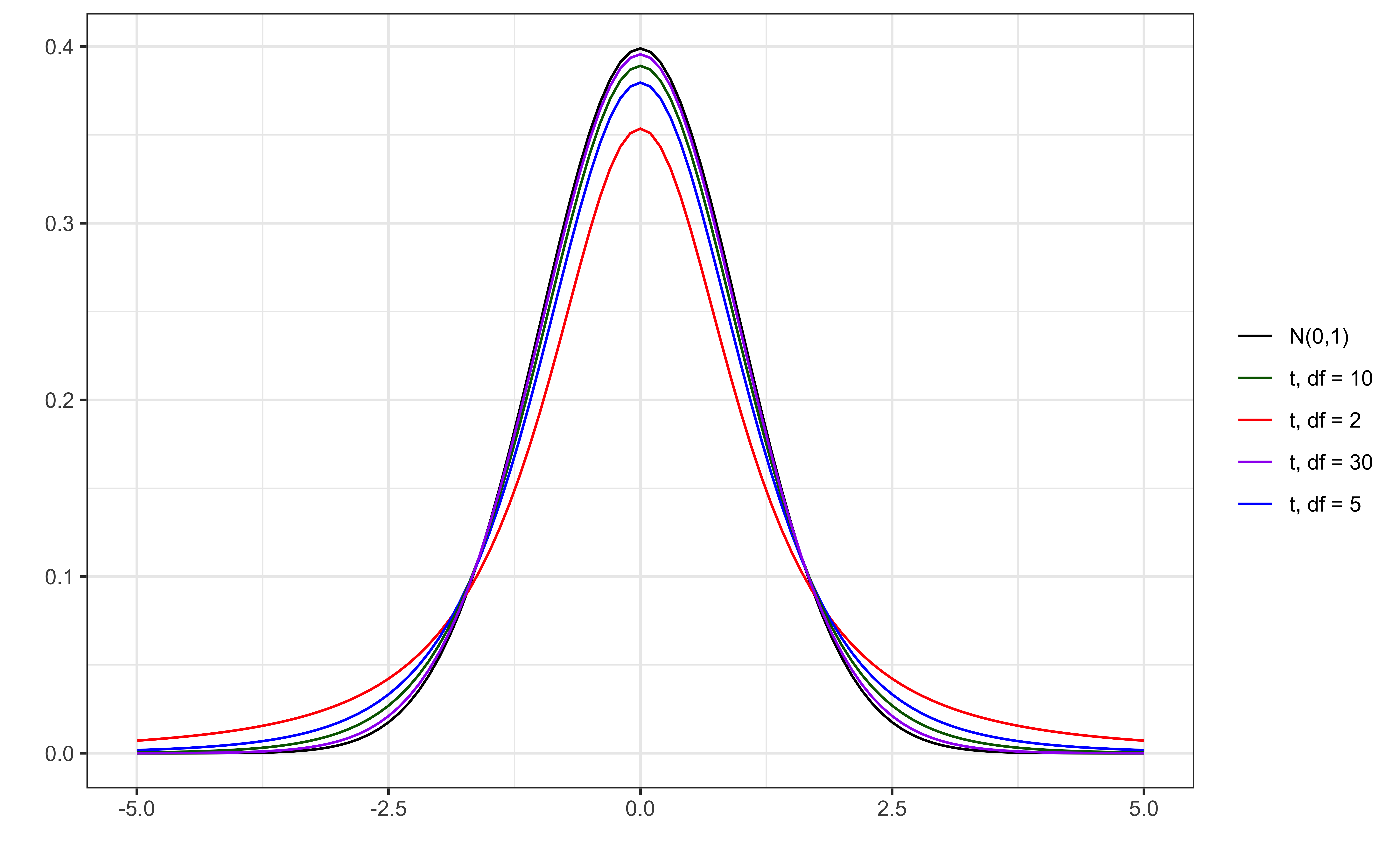
Figure 1: Standard normal vs. t distributions
Hypothesis test for \(\beta_j\): P-value
The p-value is the probability of observing a test statistic at least as extreme (in the direction of the alternative hypothesis) from the null value as the one observed
\[ p-value = P(|t| > |\text{test statistic}|), \]
calculated from a \(t\) distribution with \(n- p - 1\) degrees of freedom
Why do we take into account “extreme” on both the high and low ends?
Understanding the p-value
| Magnitude of p-value | Interpretation |
|---|---|
| p-value < 0.01 | strong evidence against \(H_0\) |
| 0.01 < p-value < 0.05 | moderate evidence against \(H_0\) |
| 0.05 < p-value < 0.1 | weak evidence against \(H_0\) |
| p-value > 0.1 | effectively no evidence against \(H_0\) |
These are general guidelines. The strength of evidence depends on the context of the problem.
Hypothesis test for \(\beta_j\): Conclusion
There are two parts to the conclusion
Make a conclusion by comparing the p-value to a predetermined decision-making threshold called the significance level ( \(\alpha\) level)
If \(\text{P-value} < \alpha\): Reject \(H_0\)
If \(\text{P-value} \geq \alpha\): Fail to reject \(H_0\)
State the conclusion in the context of the data
Application exercise
Confidence interval for \(\beta_j\)
Confidence interval for \(\beta_j\)
A plausible range of values for a population parameter is called a confidence interval
Using only a single point estimate is like fishing in a murky lake with a spear, and using a confidence interval is like fishing with a net
We can throw a spear where we saw a fish but we will probably miss, if we toss a net in that area, we have a good chance of catching the fish
Similarly, if we report a point estimate, we probably will not hit the exact population parameter, but if we report a range of plausible values we have a good shot at capturing the parameter
What “confidence” means
We will construct \(C\%\) confidence intervals.
- The confidence level impacts the width of the interval
- “Confident” means if we were to take repeated samples of the same size as our data, fit regression lines using the same predictors, and calculate \(C\%\) CIs for the coefficient of \(x_j\), then \(C\%\) of those intervals will contain the true value of the coefficient \(\beta_j\)
- Balance precision and accuracy when selecting a confidence level
Confidence interval for \(\beta_j\)
\[ \text{Estimate} \pm \text{ (critical value) } \times \text{SE} \]
\[ \hat{\beta}_1 \pm t^* \times SE({\hat{\beta}_j}) \]
where \(t^*\) is calculated from a \(t\) distribution with \(n-p-1\) degrees of freedom
Confidence interval: Critical value
95% CI for \(\beta_j\): Calculation
| term | estimate | std.error | statistic | p.value |
|---|---|---|---|---|
| (Intercept) | 19.332 | 2.984 | 6.478 | 0 |
| enrollment_th | 0.780 | 0.110 | 7.074 | 0 |
| typePublic | -13.226 | 3.153 | -4.195 | 0 |
95% CI for \(\beta_j\) in R
| term | estimate | std.error | statistic | p.value | conf.low | conf.high |
|---|---|---|---|---|---|---|
| (Intercept) | 19.332 | 2.984 | 6.478 | 0 | 13.426 | 25.239 |
| enrollment_th | 0.780 | 0.110 | 7.074 | 0 | 0.562 | 0.999 |
| typePublic | -13.226 | 3.153 | -4.195 | 0 | -19.466 | -6.986 |
Interpretation: We are 95% confident that for each additional 1,000 students enrolled, the institution’s expenditures on football will be greater by $562,000 to $999,000, on average, holding institution type constant.
Recap
Introduced statistical inference in the context of regression
Described the assumptions for regression
Connected the distribution of residuals and inferential procedures
Conducted inference on a single coefficient
Next class
- Hypothesis testing based on ANOVA