Logistic Regression: Assumptions + Estimation
Apr 10, 2025
Full model results
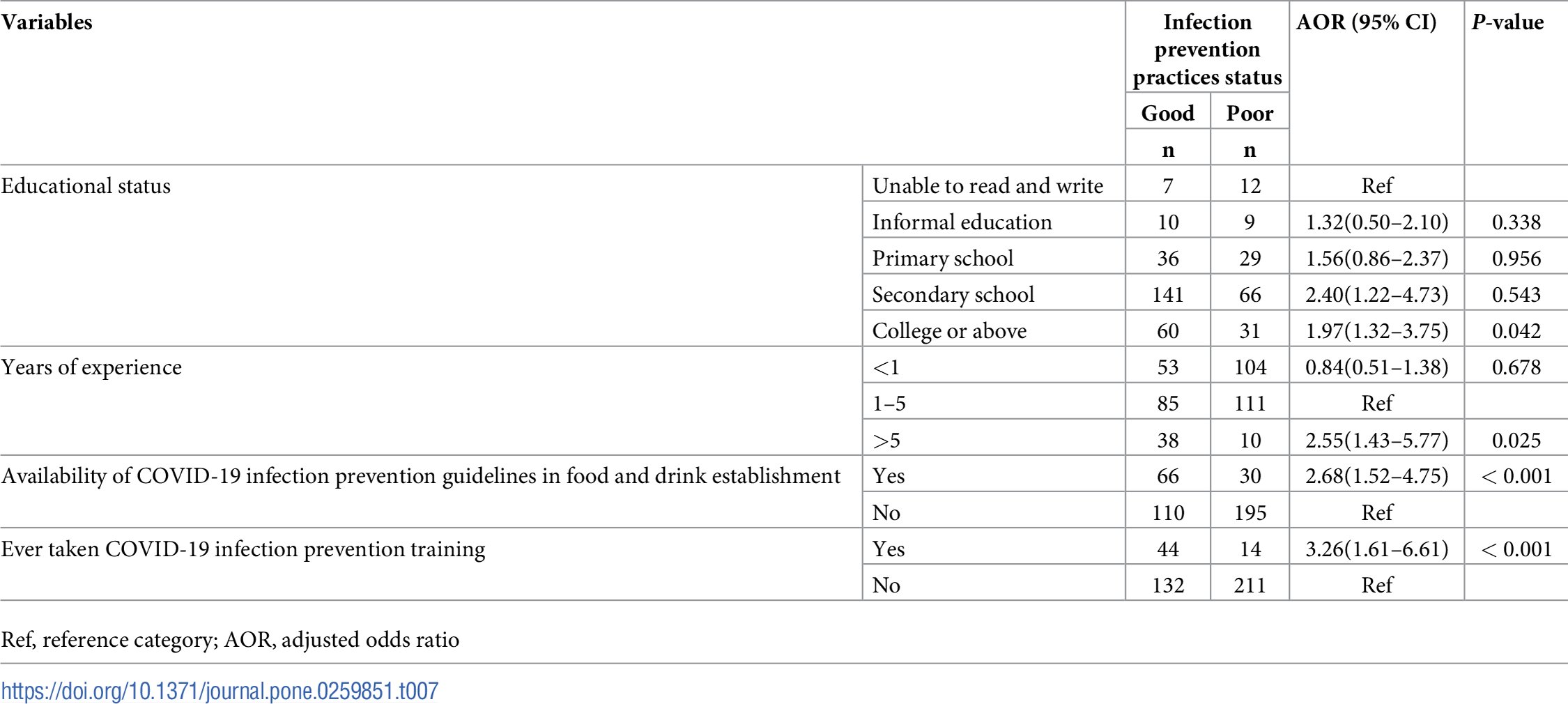
PPE Access: Interpret CI
Interpret the 95% confidence interval for > 5 years experience in terms of the odds of having access to PPE.
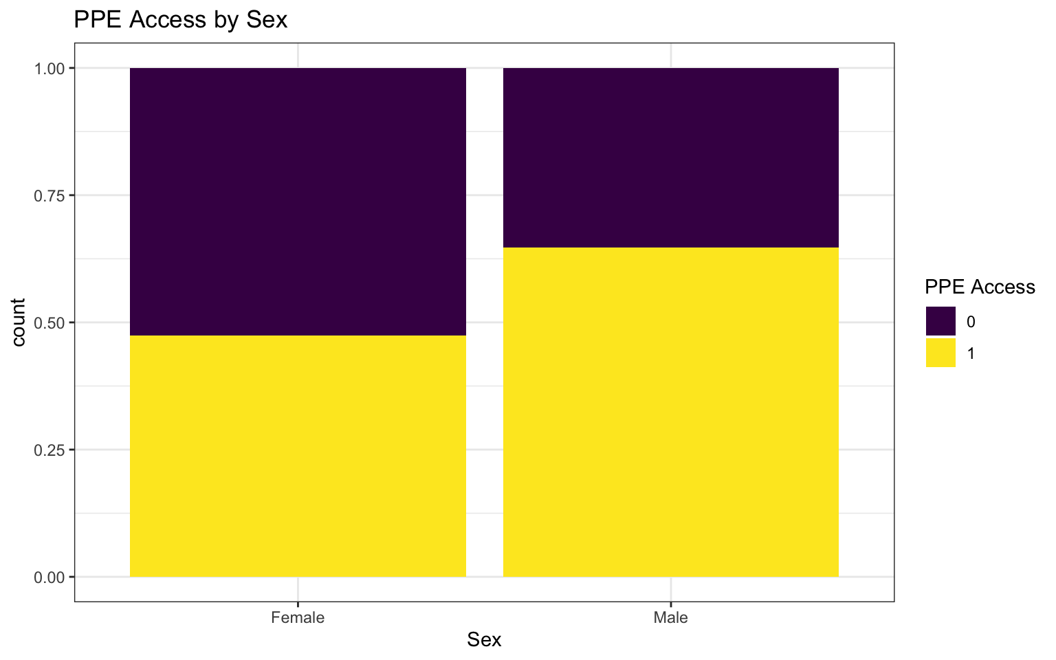
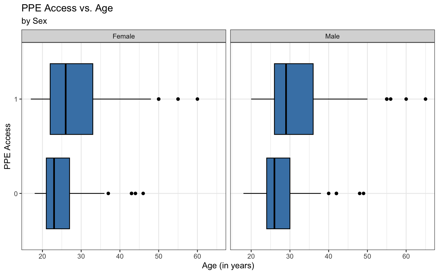
Bivariate EDA: categorical predictor
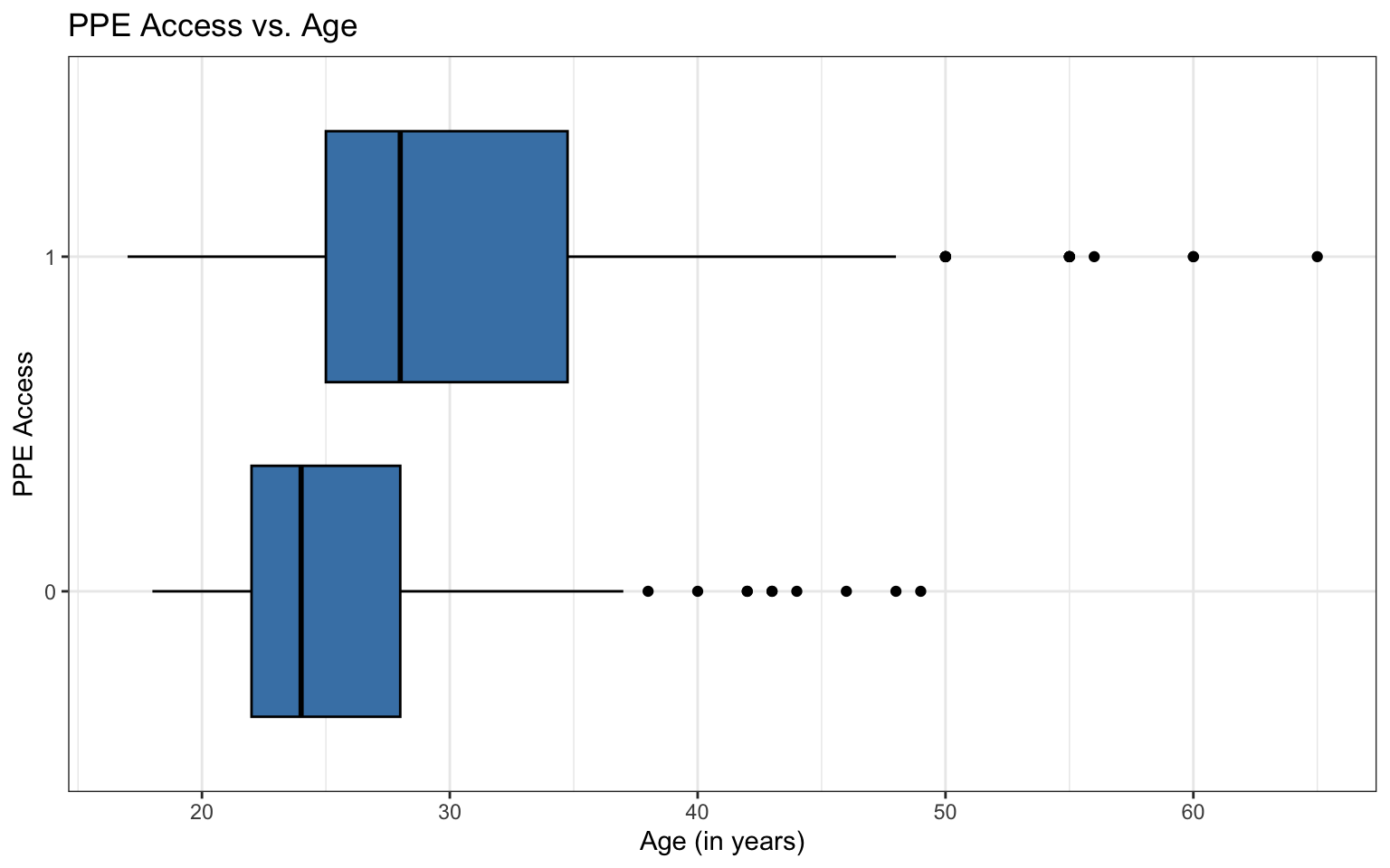
Bivariate EDA: quantitative predictor
EDA: Potential interaction effect
Empirical logit plot in R (quantitative predictor)
Created using dplyr and ggplot functions.
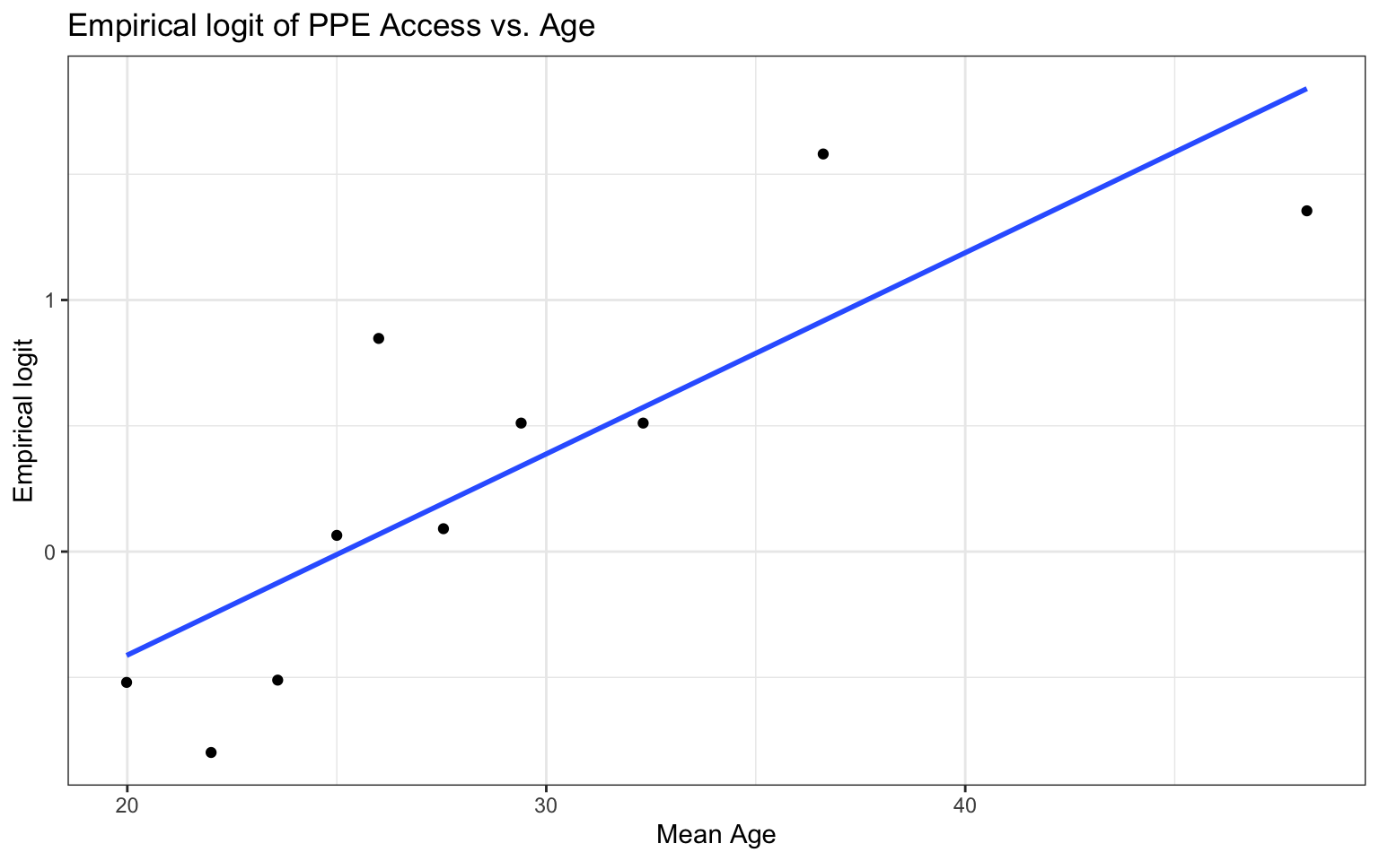
Empirical logit plot in R (quantitative predictor)
Using the emplogitplot1 function from the Stat2Data R package

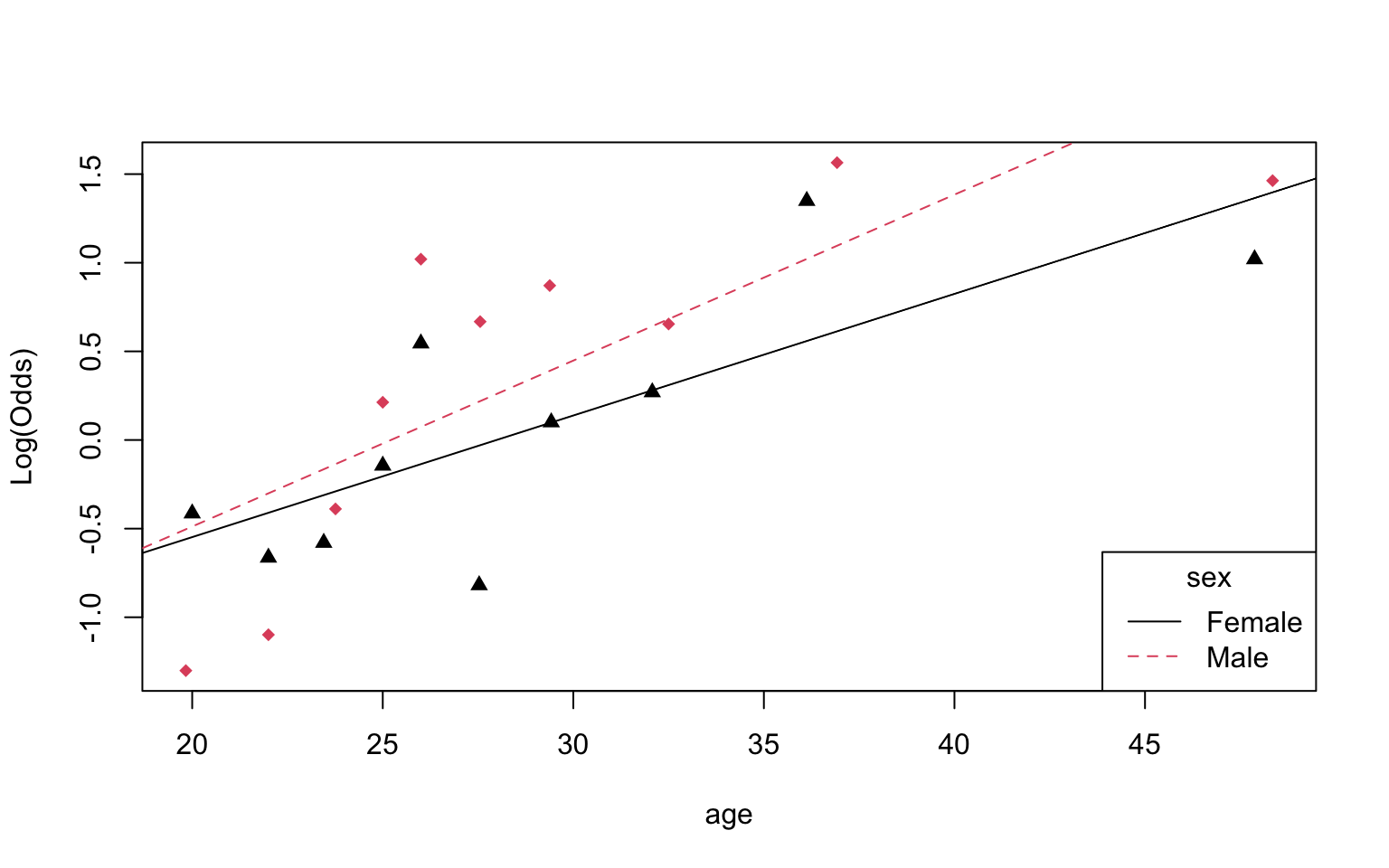
Empirical logit plot in R (interactions)
Using the emplogitplot2 function from the Stat2Data R package
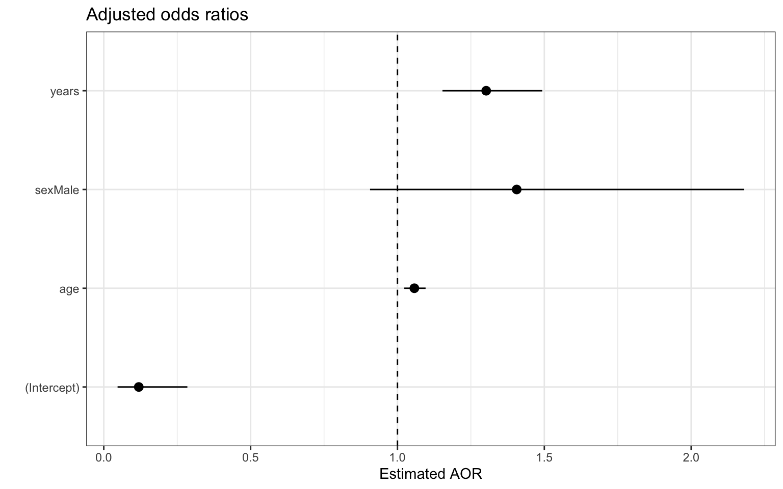
Visualizing coefficient estimates
Checking linearity
Check the empirical logit plots for the quantitative predictors
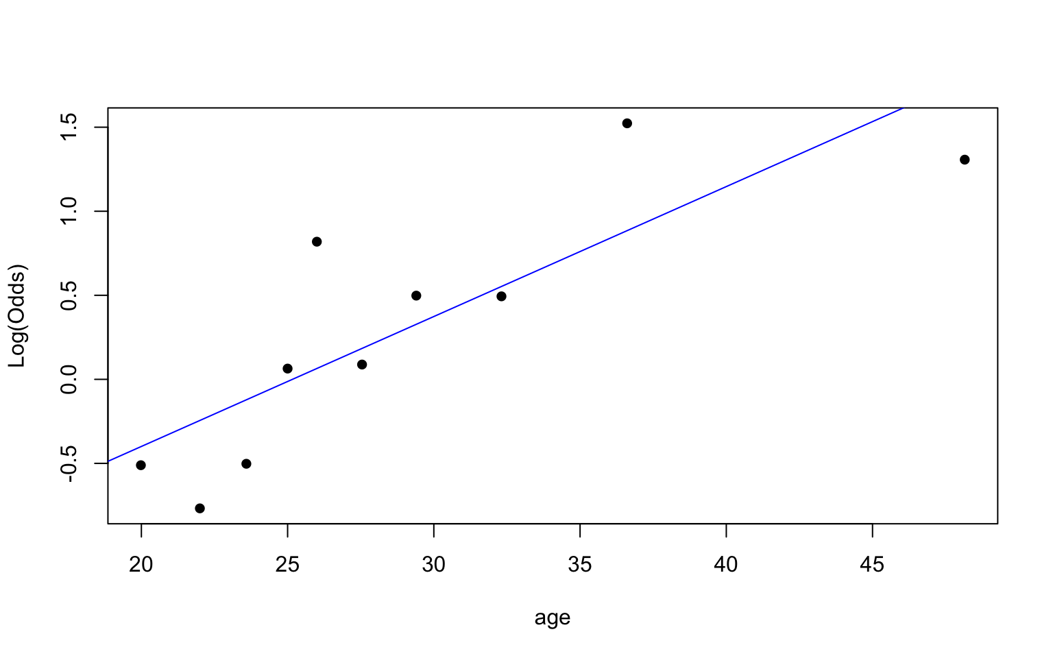
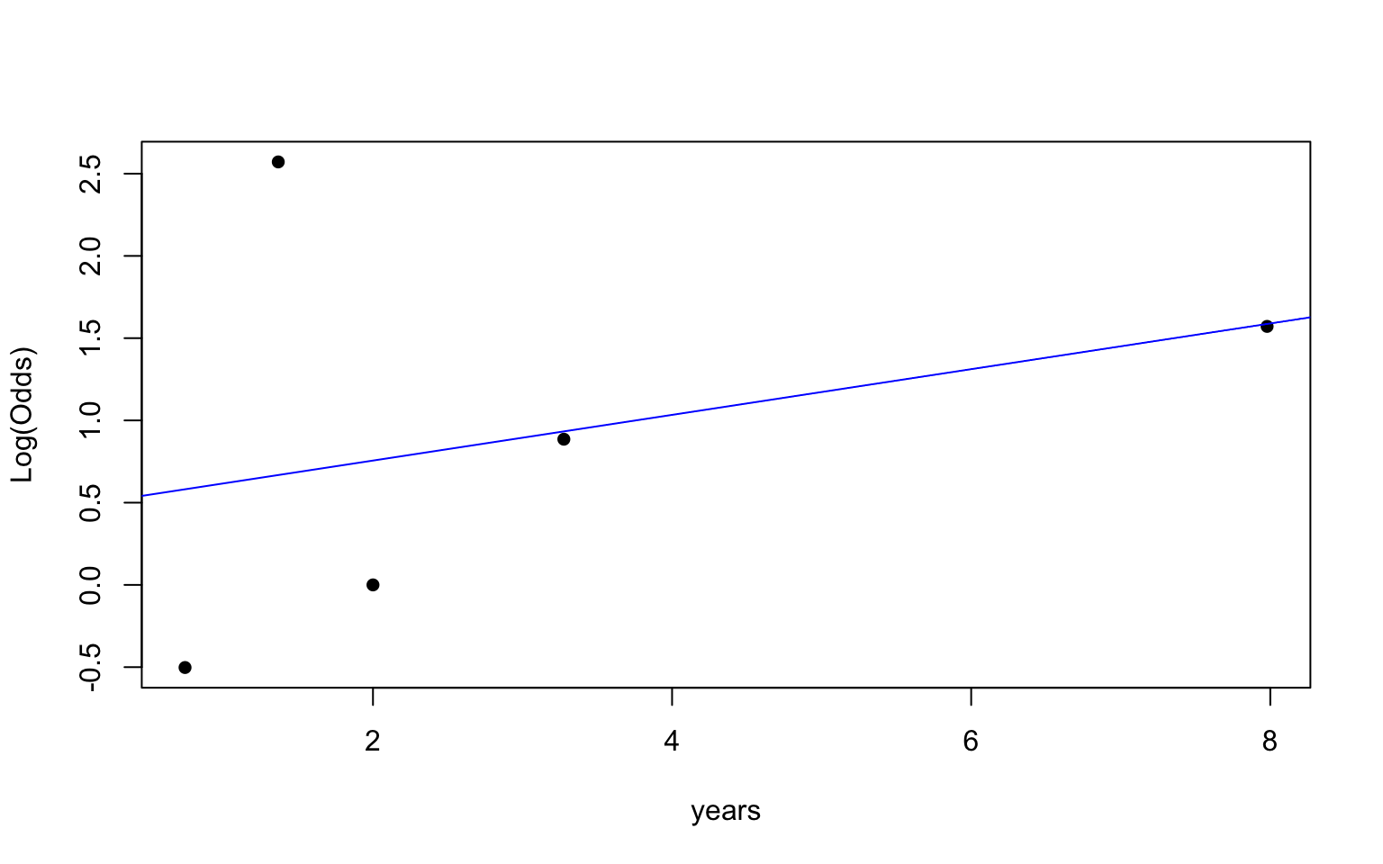
✅ The linearity condition is satisfied. There is generally a linear relationship between the empirical logit and the quantitative predictor variables
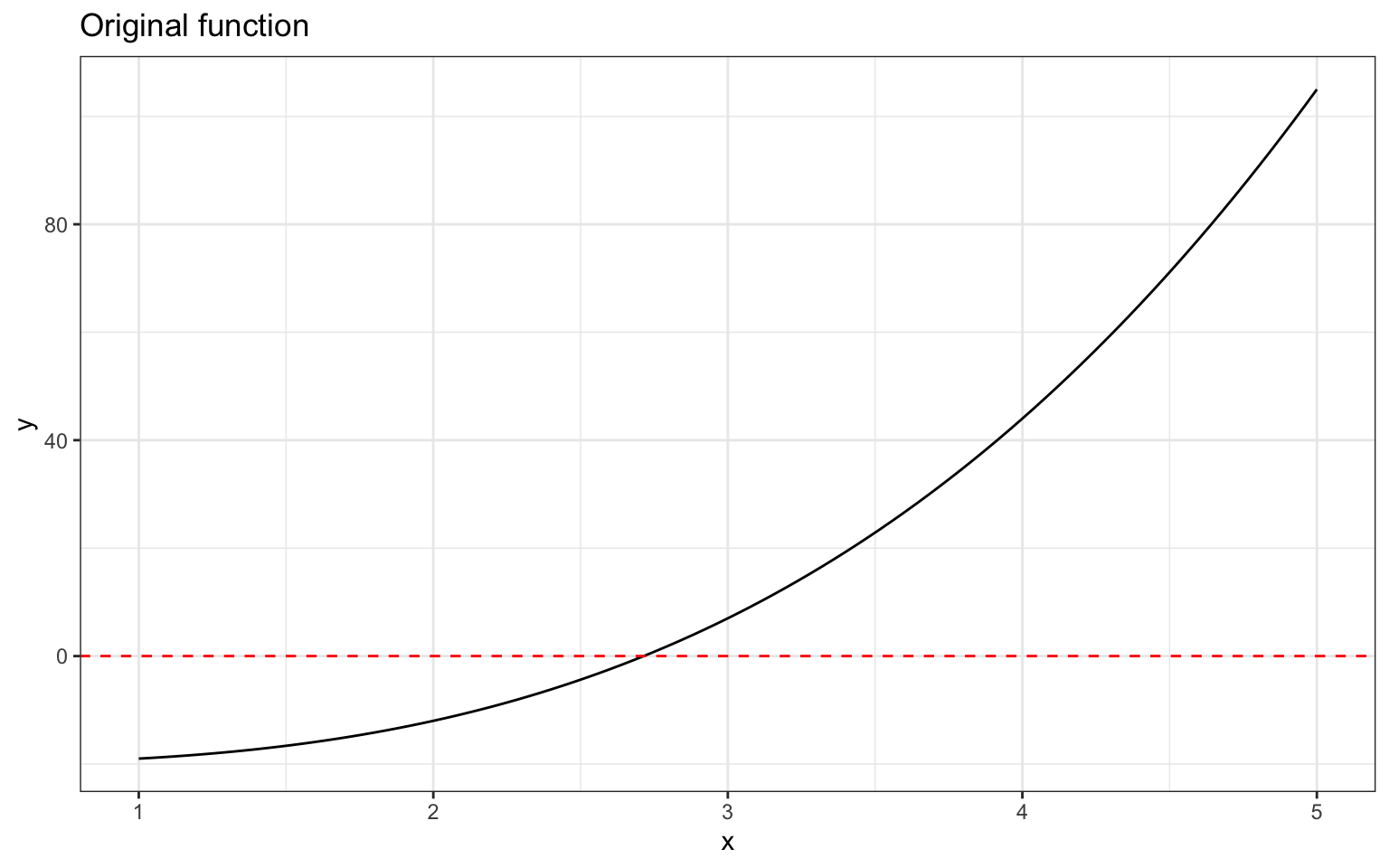
Newton-Raphson method
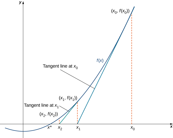
Image source: LibreTexts-Mathematics
Example
Let’s find the solution (root) of the function \[f(x) = x^3 - 20\]