Multiple linear regression

Types of predictors cont’d + Model comparison

Author

Prof. Maria Tackett

Published

Jan 30, 2025

Announcements

HW 01 due TODAY at 11:59pm
Team labs start on Friday
Click here to learn more about the Academic Resource Center
Statistics experience due Tuesday, April 22

Topics

Centering quantitative predictors
Standardizing quantitative predictors
Interaction terms
Model comparison
- RMSE
- $A d j . R^{2}$

Computing setup

# load packages
library(tidyverse)
library(tidymodels)
library(openintro)
library(patchwork)
library(knitr)
library(kableExtra)
library(viridis) #adjust color palette

# set default theme and larger font size for ggplot2
ggplot2::theme_set(ggplot2::theme_minimal(base_size = 16))

Data: Peer-to-peer lender

Today’s data is a sample of 50 loans made through a peer-to-peer lending club. The data is in the loan50 data frame in the openintro R package.

# A tibble: 50 × 4
   annual_income_th debt_to_income verified_income interest_rate
              <dbl>          <dbl> <fct>                   <dbl>
 1             59           0.558  Not Verified            10.9 
 2             60           1.31   Not Verified             9.92
 3             75           1.06   Verified                26.3 
 4             75           0.574  Not Verified             9.92
 5            254           0.238  Not Verified             9.43
 6             67           1.08   Source Verified          9.92
 7             28.8         0.0997 Source Verified         17.1 
 8             80           0.351  Not Verified             6.08
 9             34           0.698  Not Verified             7.97
10             80           0.167  Source Verified         12.6 
# ℹ 40 more rows

Variables

Predictors:

annual_income_th: Annual income (in $1000s)
debt_to_income: Debt-to-income ratio, i.e. the percentage of a borrower’s total debt divided by their total income
verified_income: Whether borrower’s income source and amount have been verified (Not Verified, Source Verified, Verified)

Response: interest_rate: Interest rate for the loan

Response vs. predictors

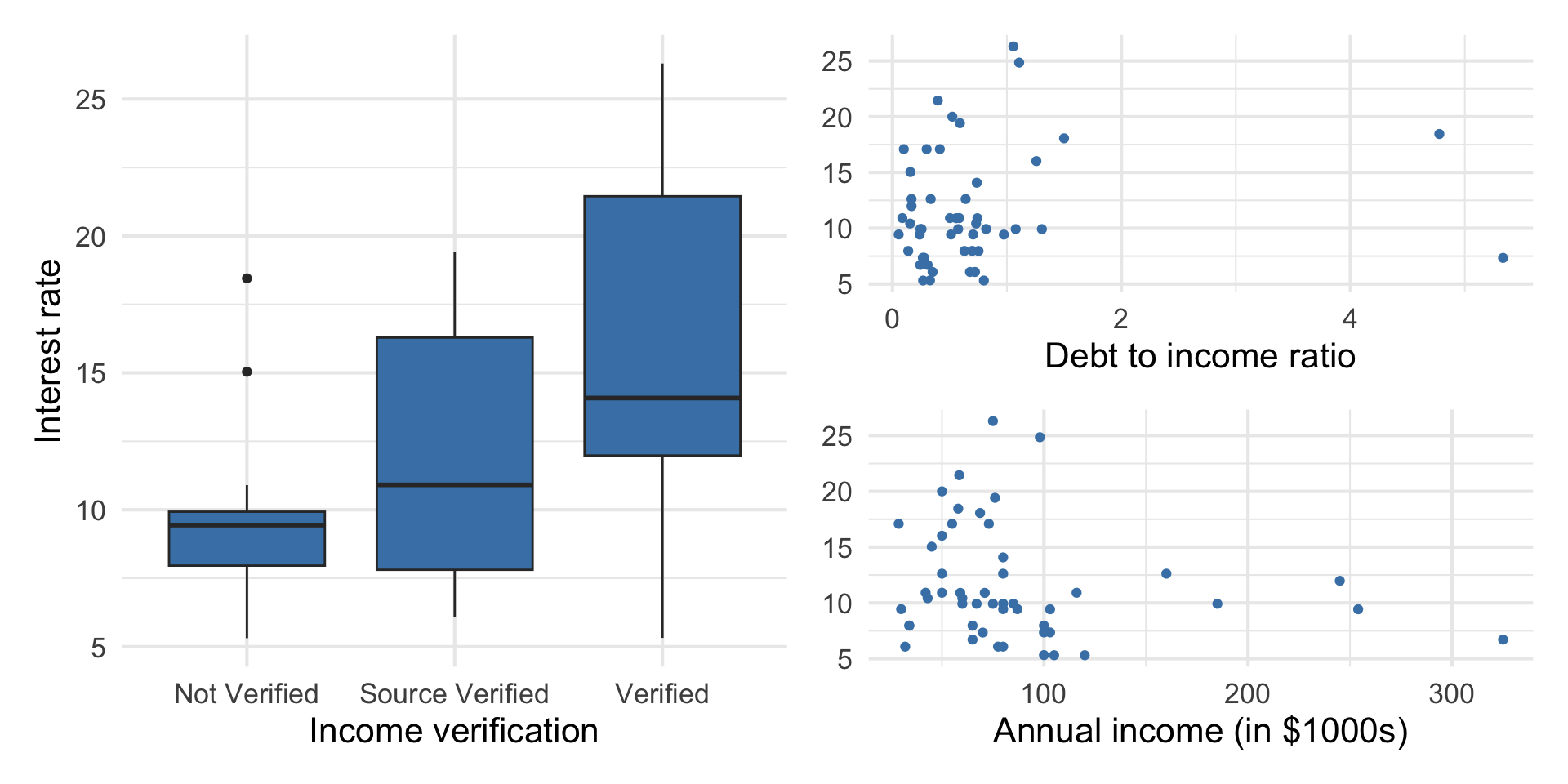
Goal: Use these predictors in a single model to understand variability in interest rate.

Model fit in R

int_fit <- lm(interest_rate ~ debt_to_income + verified_income  + annual_income_th,
              data = loan50)

tidy(int_fit) |>
  kable(digits = 3)

term	estimate	std.error	statistic	p.value
(Intercept)	10.726	1.507	7.116	0.000
debt_to_income	0.671	0.676	0.993	0.326
verified_incomeSource Verified	2.211	1.399	1.581	0.121
verified_incomeVerified	6.880	1.801	3.820	0.000
annual_income_th	-0.021	0.011	-1.804	0.078

Categorical predictors

Interpreting `verified_income`

term	estimate	std.error	statistic	p.value	conf.low	conf.high
(Intercept)	10.726	1.507	7.116	0.000	7.690	13.762
debt_to_income	0.671	0.676	0.993	0.326	-0.690	2.033
verified_incomeSource Verified	2.211	1.399	1.581	0.121	-0.606	5.028
verified_incomeVerified	6.880	1.801	3.820	0.000	3.253	10.508
annual_income_th	-0.021	0.011	-1.804	0.078	-0.043	0.002

The baseline level is Not verified.
People with source verified income are expected to take a loan with an interest rate that is 2.211% higher, on average, than the rate on loans to those whose income is not verified, holding all else constant.

Centering

Centering a quantitative predictor means shifting every value by some constant $C$

$X_{c e n t} = X - C$

One common type of centering is mean-centering, in which every value of a predictor is shifted by its mean
Only quantitative predictors are centered
Center all quantitative predictors in the model for ease of interpretation

What is one reason one might want to center the quantitative predictors? What is are the units of centered variables?

Centering

Use the scale() function with center = TRUE and scale = FALSE to mean-center variables

loan50 <- loan50 |>
  mutate(debt_to_inc_cent = scale(debt_to_income, center = TRUE, scale = FALSE), 
         annual_inc_cent = scale(annual_income_th, center = TRUE, scale = FALSE))

lm(interest_rate ~ debt_to_inc_cent + verified_income + annual_inc_cent, data = loan50) |> 
  tidy() |> kable(digits = 3)

term	estimate	std.error	statistic	p.value
(Intercept)	9.444	0.977	9.663	0.000
debt_to_inc_cent	0.671	0.676	0.993	0.326
verified_incomeSource Verified	2.211	1.399	1.581	0.121
verified_incomeVerified	6.880	1.801	3.820	0.000
annual_inc_cent	-0.021	0.011	-1.804	0.078

Centering

Term	Original Model	Centered Model
(Intercept)	10.726	9.444
debt_to_income	0.671	0.671
verified_incomeSource Verified	2.211	2.211
verified_incomeVerified	6.880	6.880
annual_income_th	-0.021	-0.021

How has the model changed? How has the model remained the same?

Standardizing

Standardizing a quantitative predictor mean shifting every value by the mean and dividing by the standard deviation of that variable

$X_{s t d} = \frac{X - \bar{X}}{S_{X}}$

Only quantitative predictors are standardized
Standardize all quantitative predictors in the model for ease of interpretation

What is one reason one might want to standardize the quantitative predictors? What is are the units of standardized variables?

Standardizing

Use the scale() function with center = TRUE and scale = TRUE to standardized variables

loan50 <- loan50 |>
  mutate(debt_to_inc_std = scale(debt_to_income, center = TRUE, scale = TRUE), 
         annual_inc_std = scale(annual_income_th, center = TRUE, scale = TRUE))

lm(interest_rate ~ debt_to_inc_std + verified_income + annual_inc_std, data = loan50) |>
  tidy() |> kable(digits = 3)

term	estimate	std.error	statistic	p.value
(Intercept)	9.444	0.977	9.663	0.000
debt_to_inc_std	0.643	0.648	0.993	0.326
verified_incomeSource Verified	2.211	1.399	1.581	0.121
verified_incomeVerified	6.880	1.801	3.820	0.000
annual_inc_std	-1.180	0.654	-1.804	0.078

Standardizing

Term	Original Model	Standardized Model
(Intercept)	10.726	9.444
debt_to_income	0.671	0.643
verified_incomeSource Verified	2.211	2.211
verified_incomeVerified	6.880	6.880
annual_income_th	-0.021	-1.180

How has the model changed? How has the model remained the same?

Interaction terms

Sometimes the relationship between a predictor variable and the response depends on the value of another predictor variable.
This is an interaction effect.
To account for this, we can include interaction terms in the model.

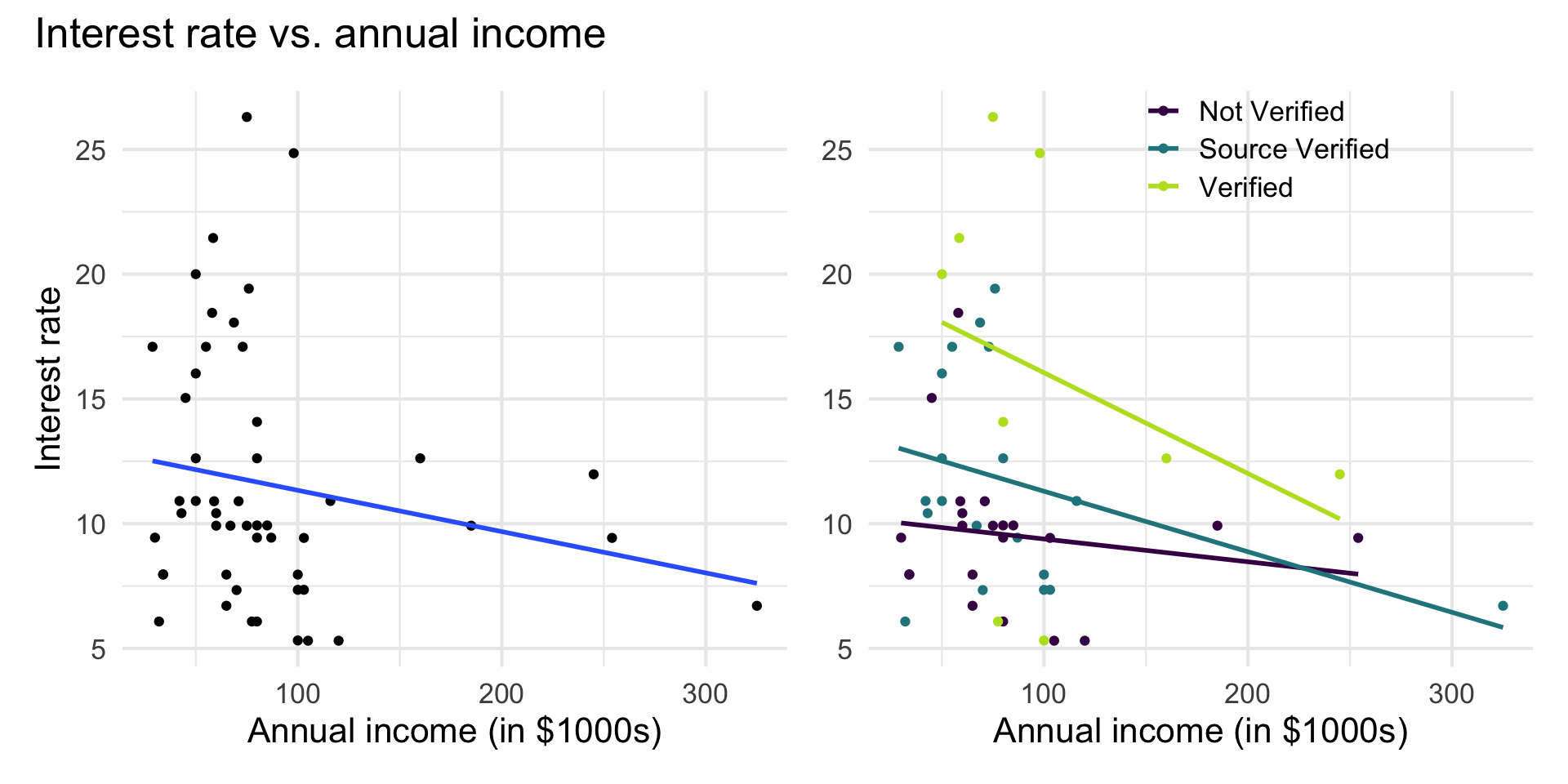
Interest rate vs. annual income

The lines are not parallel indicating there is a potential interaction effect. The slope of annual income potentially differs based on the income verification.

Interaction term in model

int_fit_2 <- lm(interest_rate ~ debt_to_income + verified_income + annual_income_th + verified_income * annual_income_th,
      data = loan50)

term	estimate	std.error	statistic	p.value
(Intercept)	9.560	2.034	4.700	0.000
debt_to_income	0.691	0.685	1.009	0.319
verified_incomeSource Verified	3.577	2.539	1.409	0.166
verified_incomeVerified	9.923	3.654	2.716	0.009
annual_income_th	-0.007	0.020	-0.341	0.735
verified_incomeSource Verified:annual_income_th	-0.016	0.026	-0.643	0.523
verified_incomeVerified:annual_income_th	-0.032	0.033	-0.979	0.333

Interaction term in model

term	estimate	std.error	statistic	p.value
(Intercept)	9.560	2.034	4.700	0.000
debt_to_income	0.691	0.685	1.009	0.319
verified_incomeSource Verified	3.577	2.539	1.409	0.166
verified_incomeVerified	9.923	3.654	2.716	0.009
annual_income_th	-0.007	0.020	-0.341	0.735
verified_incomeSource Verified:annual_income_th	-0.016	0.026	-0.643	0.523
verified_incomeVerified:annual_income_th	-0.032	0.033	-0.979	0.333

Write the regression equation for the people with Not Verified income.
Write the regression equation for people with Verified income.

Interpreting interaction terms

What the interaction means: The effect of annual income on the interest rate differs by -0.016 when the income is source verified compared to when it is not verified, holding all else constant.
Interpreting annual_income for source verified: If the income is source verified, we expect the interest rate to decrease by 0.023% (-0.007 + -0.016) for each additional thousand dollars in annual income, holding all else constant.

Summary

In general, how do

indicators for categorical predictors impact the model equation?
interaction terms impact the model equation?

Model comparison

Model assessment: RMSE & $R^{2}$

Root mean square error, RMSE: A measure of the average error (average difference between observed and predicted values of the outcome)
R-squared, $R^{2}$ : Percentage of variability in the outcome explained by the regression model

Comparing models

When comparing models, do we prefer the model with the lower or higher RMSE?
Though we use $R^{2}$ to assess the model fit, it is generally unreliable for comparing models with different number of predictors. Why?
- $R^{2}$ will stay the same or increase as we add more variables to the model . Let’s show why this is true.
- If we only use $R^{2}$ to choose a best fit model, we will be prone to choose the model with the most predictor variables.

Adjusted $R^{2}$

Adjusted $R^{2}$ : measure that includes a penalty for unnecessary predictor variables
Similar to $R^{2}$ , it is a measure of the amount of variation in the response that is explained by the regression model
Use the glance() function to get $A d j . R^{2}$ in R

glance(int_fit)$adj.r.squared

[1] 0.215841

$R^{2}$ and Adjusted $R^{2}$

$R^{2} = \frac{S S M}{S S T} = 1 - \frac{S S R}{S S T}$

. . .

$R_{a d j}^{2} = 1 - \frac{S S R / (n - p - 1)}{S S T / (n - 1)}$

where

$n$ is the number of observations used to fit the model
$p$ is the number of terms (not including the intercept) in the model

Using $R^{2}$ and Adjusted $R^{2}$

Adjusted $R^{2}$ can be used as a quick assessment to compare the fit of multiple models; however, it should not be the only assessment!
Use $R^{2}$ when describing the relationship between the response and predictor variables

Comparing interest rate models

Model without interaction

# r-squared
glance(int_fit)$r.squared

[1] 0.279854

# adj-r-squared
glance(int_fit)$adj.r.squared

[1] 0.215841

Model with interaction

# r-squared
glance(int_fit_2)$r.squared

[1] 0.2963437

# adj-r-squared
glance(int_fit_2)$adj.r.squared

[1] 0.1981591

Recap

Fit and interpreted models with centered and standardized variables
Interpreted interaction terms
Used RMSE and $A d j . R^{2}$ to compare models

Next class

Inference for regression
See Prepare for Lecture 08

Announcements

Topics

Computing setup

Data: Peer-to-peer lender

Variables

Response vs. predictors

Model fit in R

Categorical predictors

Interpreting verified_income

Centering

Centering

Centering

Standardizing

Standardizing

Standardizing

Interaction terms

Interaction terms

Interest rate vs. annual income

Interaction term in model

Interaction term in model

Interpreting interaction terms

Summary

Model comparison

Model assessment: RMSE & R2

Comparing models

Adjusted R2

R2 and Adjusted R2

Using R2 and Adjusted R2

Comparing interest rate models

Recap

Next class

Interpreting `verified_income`

Model assessment: RMSE & $R^{2}$

Adjusted $R^{2}$

$R^{2}$ and Adjusted $R^{2}$

Using $R^{2}$ and Adjusted $R^{2}$