Model conditions + diagnostics

Announcements

• Exam corrections (optional) due Tuesday, March 4 at 11:59pm

  • See assignment on Canvas

• Project proposal due TODAY at 11:59pm

Computing set up

# load packages
library(tidyverse)  
library(tidymodels)  
library(knitr)       
library(patchwork)   
library(viridis)

# set default theme in ggplot2
ggplot2::theme_set(ggplot2::theme_bw(base_size = 16))

Topics

• Model conditions

• Influential points

• Model diagnostics

  • Leverage

  • Studentized residuals

  • Cook’s Distance

Data: Duke lemurs

Today’s data contains a subset of the original Duke Lemur data set available in the TidyTuesday GitHub repo. This data includes information on “young adult” lemurs from the Coquerel’s sifaka species (PCOQ), the largest species at the Duke Lemur Center. The analysis will focus on the following variables:

• age_at_wt_mo: Age in months: Age of the animal when the weight was taken, in months (((Weight_Date-DOB)/365)*12)

• weight_g: Weight: Animal weight, in grams. Weights under 500g generally to nearest 0.1-1g; Weights >500g generally to the nearest 1-20g.

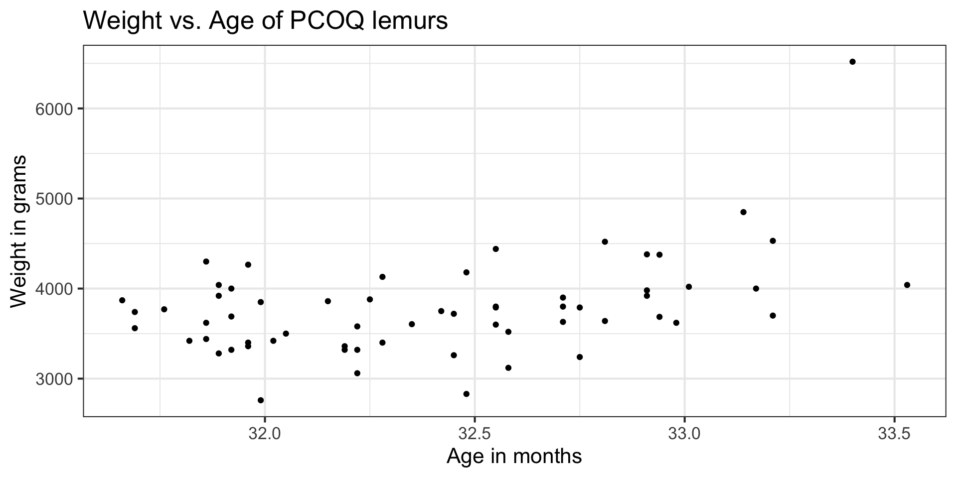
The goal of the analysis is to use the age of the lemurs to understand variability in the weight.

EDA

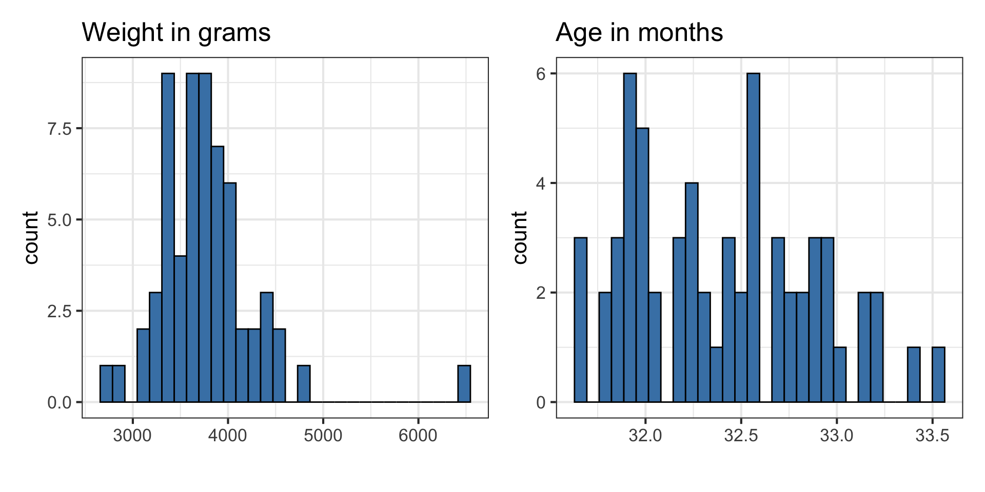
EDA

Fit model

lemurs_fit <- lm(weight_g ~ age_at_wt_mo, data = lemurs)

tidy(lemurs_fit) |> 
  kable(digits = 3)

term	estimate	std.error	statistic	p.value
(Intercept)	-12314.360	4252.696	-2.896	0.005
age_at_wt_mo	496.591	131.225	3.784	0.000

Model conditions

Assumptions for regression

$$\mathbf{y}|\mathbf{X}\sim N(\mathbf{X}\mathit{\beta },{\sigma }_{ϵ}^2\mathbf{I})$$

1. Linearity: There is a linear relationship between the response and predictor variables.
2. Constant Variance: The variability about the least squares line is generally constant.
3. Normality: The distribution of the errors (residuals) is approximately normal.
4. Independence: The errors (residuals) are independent from one another.

. . .

How do we know if these assumptions hold in our data?

Linearity

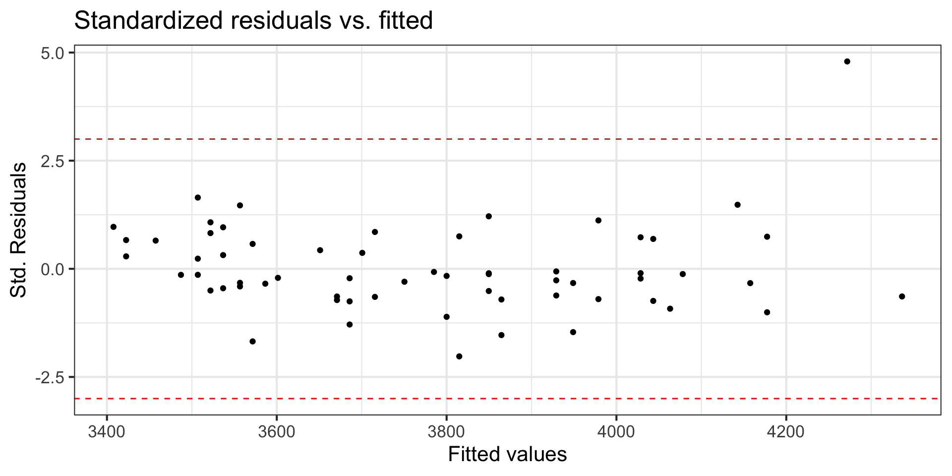
• Look at plot of residuals versus fitted (predicted) values.
• Linearity is satisfied if there is no discernible pattern in the plot (i.e., points randomly scattered around $residuals=0$

. . .

. . .

Linearity is satisfied

Example: Linearity not satisfied

. . .

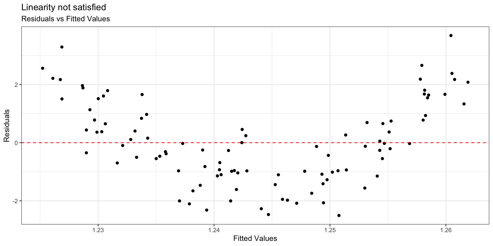
• If linearity is not satisfied, examine the plots of residuals versus each predictor.
• Add higher order term(s), as needed.

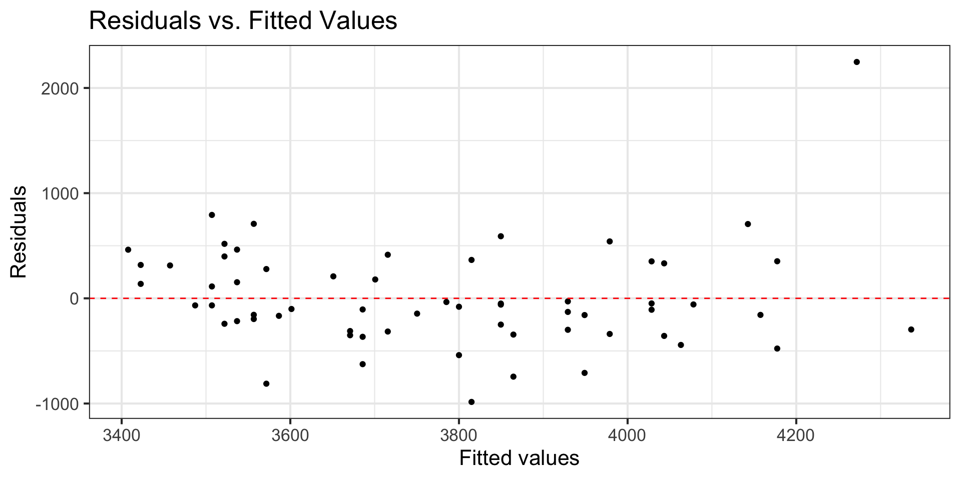
Constant variance

• Look at plot of residuals versus fitted (predicted) values.
• Constant variance is satisfied if the vertical spread of the points is approximately equal for all fitted values

. . .

. . .

Constant variance is satisfied

Example: Constant variance not satisfied

. . .

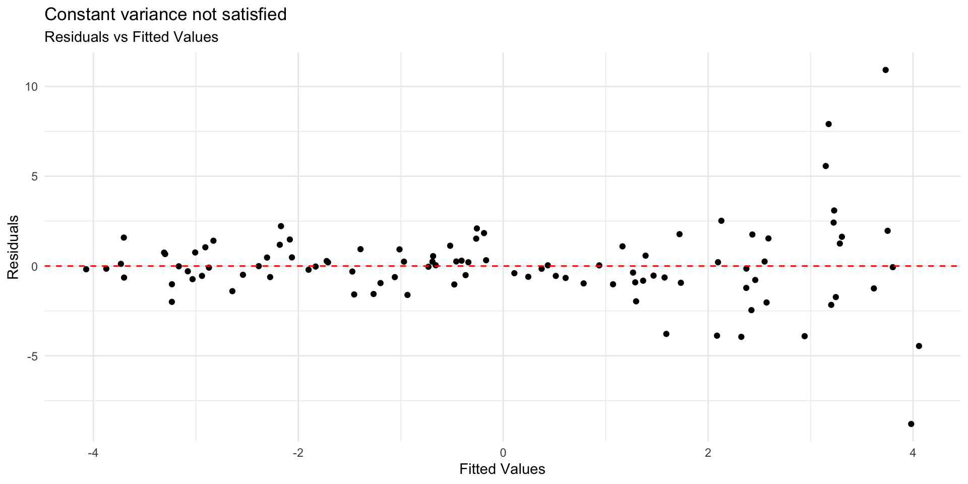
• Constant variance is critical for reliable inference

• Address violations by applying transformation on the response

Normality

• Look at the distribution of the residuals
• Normality is satisfied if the distribution is approximately unimodal and symmetric. Inference robust to violations if $n>30$

. . .

Distribution approximately unimodal and symmetric, aside from the outlier. There are 62 observations, so inference robust to departures.

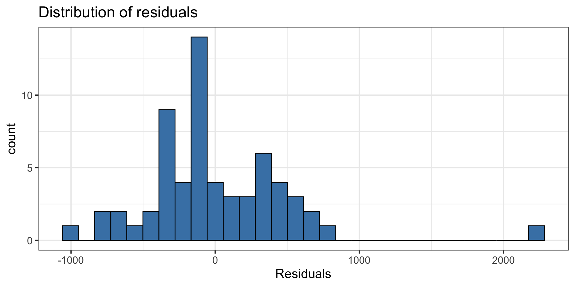
Independence

• We can often check the independence condition based on the context of the data and how the observations were collected.

• If the data were collected in a particular order, examine a scatterplot of the residuals versus order in which the data were collected.

• If data has spatial element, plot residuals on a map to examine potential spatial correlation.

. . .

The independence condition is satisfied. The lemurs could reasonably be treated as independent.

Model diagnostics

Model diagnostics

lemurs_aug <- augment(lemurs_fit)

lemurs_aug |> slice(1:10)

# A tibble: 10 × 8
   weight_g age_at_wt_mo .fitted .resid   .hat .sigma  .cooksd .std.resid
      <dbl>        <dbl>   <dbl>  <dbl>  <dbl>  <dbl>    <dbl>      <dbl>
 1     3400         32.0   3557. -157.  0.0302   494. 0.00164      -0.324
 2     3620         33.0   4063. -443.  0.0399   491. 0.0176       -0.922
 3     3720         32.4   3800.  -80.0 0.0163   495. 0.000224     -0.164
 4     4440         32.6   3850.  590.  0.0177   489. 0.0132        1.21 
 5     3770         31.8   3457.  313.  0.0458   493. 0.0102        0.652
 6     3920         31.9   3522.  398.  0.0350   492. 0.0124        0.826
 7     4520         32.8   3979.  541.  0.0279   490. 0.0180        1.12 
 8     3700         33.2   4177. -477.  0.0626   491. 0.0337       -1.01 
 9     3690         31.9   3537.  153.  0.0329   494. 0.00172       0.318
10     3790         32.8   3949. -159.  0.0247   494. 0.00136      -0.328

Model diagnostics in R

Use the augment() function in the broom package to output the model diagnostics (along with the predicted values and residuals)

• response and predictor variables in the model
• .fitted: predicted values
• .se.fit: standard errors of predicted values
• .resid: residuals
• .hat: leverage
• .sigma: estimate of residual standard deviation when the corresponding observation is dropped from model
• .cooksd: Cook’s distance
• .std.resid: standardized residuals

Influential Point

An observation is influential if removing has a noticeable impact on the regression coefficients

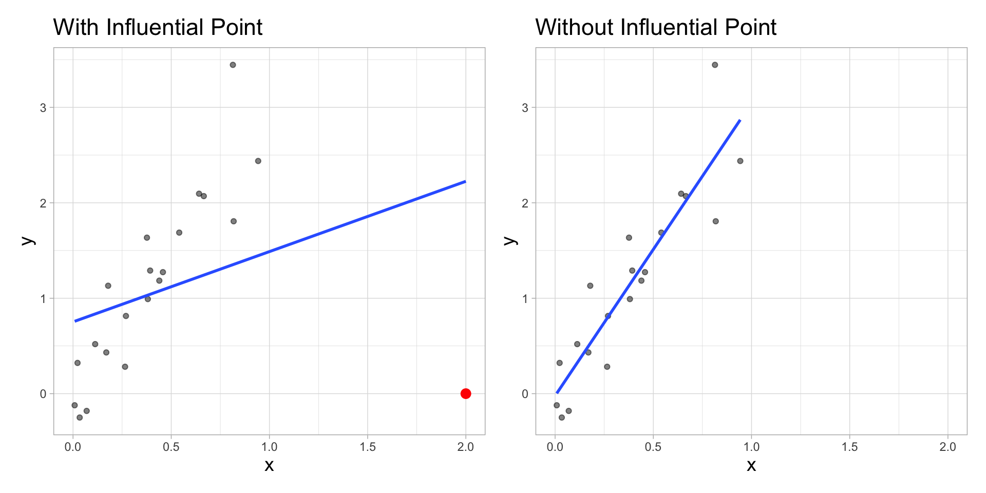
Influential points

• Influential points have a noticeable impact on the coefficients and standard errors used for inference
• These points can sometimes be identified in a scatterplot if there is only one predictor variable
  • This is often not the case when there are multiple predictors
• We will use measures to quantify an individual observation’s influence on the regression model
  • leverage, standardized & studentized residuals, and Cook’s distance

Cook’s Distance

Motivating Cook’s Distance

• An observation’s influence on the regression line depends on

  • How close it lies to the general trend of the data

  • Its leverage

• Cook’s Distance is a statistic that includes both of these components to measure an observation’s overall impact on the model

Cook’s Distance

Cook’s distance for the $i^{th}$ observation is

$$D_i=\frac{r_i^2}{p+1}(\frac{h_{ii}}{1-h_{ii}})$$

where $r_i$ is the studentized residual and $h_{ii}$ is the leverage for the $i^{th}$ observation

. . .

This measure is a combination of

• How well the model fits the $i^{th}$ observation (magnitude of residuals)

• How far the $i^{th}$ observation is from the rest of the data (where the point is in the $x$ space)

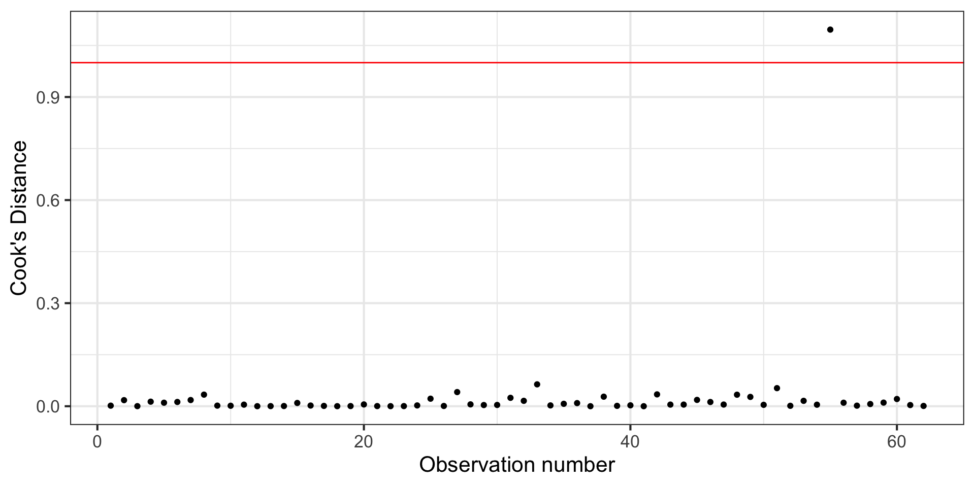
Using Cook’s Distance

• An observation with large value of $D_i$ is said to have a strong influence on the predicted values

• General thresholds .An observation with

  • $D_i>0.5$ is moderately influential

  • $D_i>1$ is very influential

Cook’s Distance

Cook’s Distance is in the column .cooksd in the output from the augment() function

Comparing models

With influential point

term	estimate	std.error	statistic	p.value
(Intercept)	-12314.360	4252.696	-2.896	0.005
age_at_wt_mo	496.591	131.225	3.784	0.000

Without influential point

term	estimate	std.error	statistic	p.value
(Intercept)	-6670.958	3495.136	-1.909	0.061
age_at_wt_mo	321.209	107.904	2.977	0.004

. . .

Let’s better understand the influential point.

Leverage

Leverage

• Recall the hat matrix $\mathbf{H}=\mathbf{X}({\mathbf{X}}^{\mathsf{T}}\mathbf{X}{)}^{-1}{\mathbf{X}}^{\mathsf{T}}$

• We focus on the diagonal elements

  $$h_{ii}={\mathbf{x}}_i^{\mathsf{T}}({\mathbf{X}}^{\mathsf{T}}\mathbf{X}{)}^{-1}{\mathbf{x}}_i$$such that ${\mathbf{x}}_i^{\mathsf{T}}$ is the $i^{th}$ row of $\mathbf{X}$

• $h_{ii}$ is the leverage: a measure of the distance of the $i^{th}$ observation from the center (or centroid) of the $x$ space

• Observations with large values of $h_{ii}$ are far away from the typical value (or combination of values) of the predictors in the data

Large leverage

• The sum of the leverages for all points is $p+1$, where $p$ is the number of predictors in the model . More specifically

  $$\sum _{i=1}^n{h}_{ii}=\text{rank}(\mathbf{H})=\text{rank}(\mathbf{X})=p+1$$

• The average value of leverage, $h_{ii}$, is $\overline{h}=\frac{(p+1)}{n}$

• An observation has large leverage if $$h_{ii}>\frac{2(p+1)}{n}$$

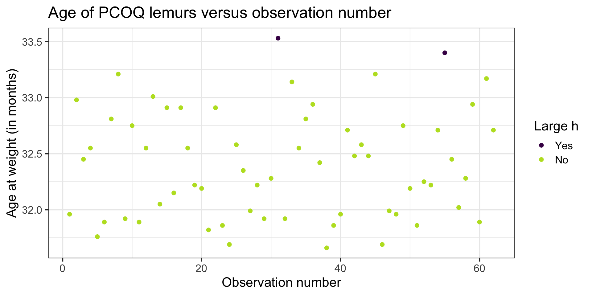
Lemurs: Leverage

h_threshold <- 2 * 2 / nrow(lemurs)
h_threshold

[1] 0.06451613

. . .

lemurs_aug |>
  filter(.hat > h_threshold)

# A tibble: 2 × 8
  weight_g age_at_wt_mo .fitted .resid   .hat .sigma .cooksd .std.resid
     <dbl>        <dbl>   <dbl>  <dbl>  <dbl>  <dbl>   <dbl>      <dbl>
1     4040         33.5   4336.  -296. 0.107    493.  0.0244     -0.639
2     6519         33.4   4272.  2247. 0.0871   389.  1.10        4.79 

. . .

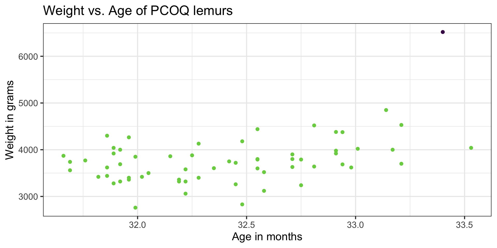
Why do you think these points have large leverage?

Let’s look at the data

Large leverage

If there is point with high leverage, ask

• ❓ Is there a data entry error?

• ❓ Is this observation within the scope of individuals for which you want to make predictions and draw conclusions?

• ❓ Is this observation impacting the estimates of the model coefficients? (Need more information!)

. . .

Just because a point has high leverage does not necessarily mean it will have a substantial impact on the regression. Therefore we need to check other measures.

Scaled residuals

Scaled residuals

• What is the best way to identify outlier points that don’t fit the pattern from the regression line?

  • Look for points that have large residuals

• We can rescale residuals and put them on a common scale to more easily identify “large” residuals

• We will consider two types of scaled residuals: standardized residuals and studentized residuals

Standardized residuals

• The variance of the residuals can be estimated by the mean squared residuals (MSR) $=\frac{SSR}{n-p-1}={\hat{\sigma }}_{ϵ}^2$

• We can use MSR to compute standardized residuals

  $$std.re{s}_i=\frac{e_i}{\sqrt{MSR}}$$

• Standardized residuals are produced by augment() in the column .std.resid

---

Using standardized residuals

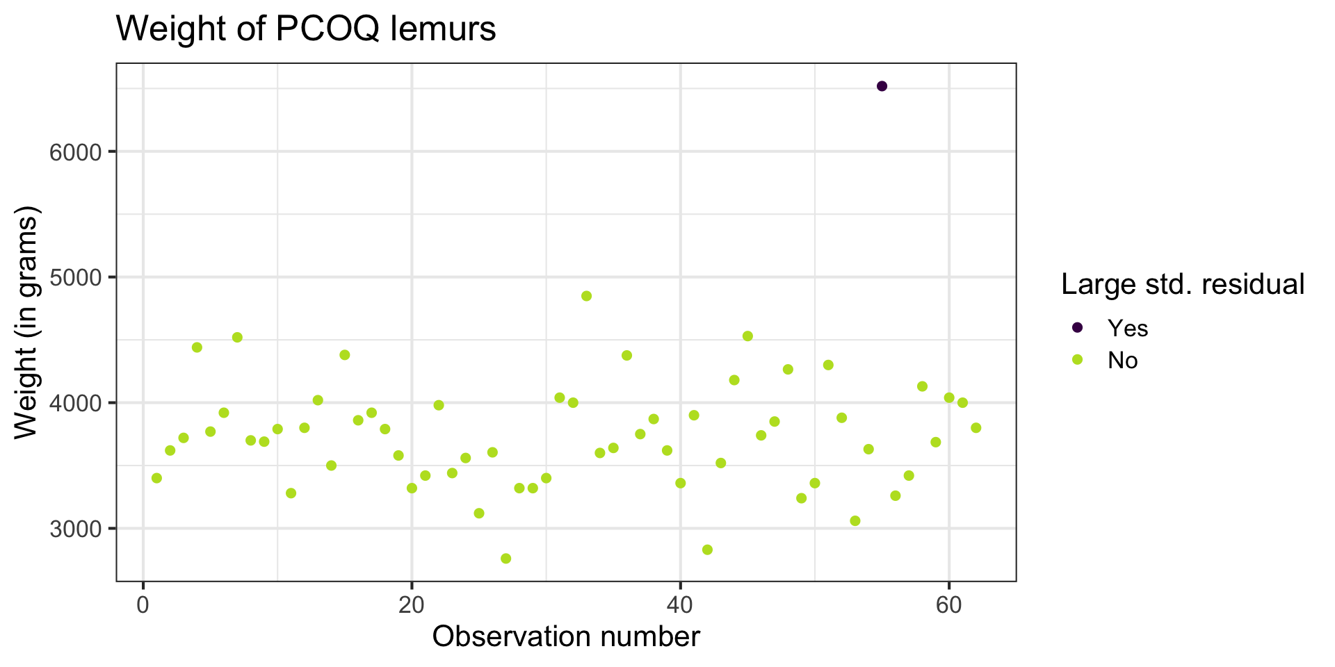
We can examine the standardized residuals directly from the output from the augment() function

• An observation is a potential outlier if its standardized residual is beyond $\pm 3$

Digging in to the data

Let’s look at the value of the response variable to better understand potential outliers

Studentized residuals

• MSR is an approximation of the variance of the residuals.

• The variance of the residuals is $Var(\mathbf{e})={\sigma }_{ϵ}^2(\mathbf{I}-\mathbf{H})$

  • The variance of the $i^{th}$ residual is $Var(e_i)={\sigma }_{ϵ}^2(1-h_{ii})$

• The studentized residual is the residual rescaled by the more exact calculation for variance

$$r_i=\frac{e_i}{\sqrt{{\hat{\sigma }}_{ϵ}^2(1-h_{ii})}}$$

• Standardized and studentized residuals provide similar information about which points are outliers in the response.
  • Studentized residuals are used to compute Cook’s Distance.

Using these measures

• Standardized residuals, leverage, and Cook’s Distance should all be examined together

• Examine plots of the measures to identify observations that are outliers, high leverage, and may potentially impact the model.

Back to the influential point

What to do with outliers/influential points?

• First consider if the outlier is a result of a data entry error.

• If not, you may consider dropping an observation if it’s an outlier in the predictor variables if…

  • It is meaningful to drop the observation given the context of the problem

  • You intended to build a model on a smaller range of the predictor variables. Mention this in the write up of the results and be careful to avoid extrapolation when making predictions

What to do with outliers/influential points?

• It is generally not good practice to drop observations that ar outliers in the value of the response variable

  • These are legitimate observations and should be in the model

  • You can try transformations or increasing the sample size by collecting more data

• A general strategy when there are influential points is to fit the model with and without the influential points and compare the outcomes

---

Recap

• Model conditions

• Influential points

• Model diagnostics

  • Leverage

  • Studentized residuals

Cook’s Distance