Multicollinearity

Author

Prof. Maria Tackett

Published

Feb 27, 2025

Announcements

Exam corrections (optional) due Tuesday, March 4 at 11:59pm
- See assignment on Canvas
Team Feedback (email from TEAMMATES) due Tuesday, March 4 at 11:59pm (check email)
DataFest: April 4 - 6 - https://dukestatsci.github.io/datafest/

Computing set up

# load packages
library(tidyverse)  
library(tidymodels)  
library(knitr)       
library(patchwork)
library(GGally)   # for pairwise plot matrix
library(corrplot) # for correlation matrix

# set default theme in ggplot2
ggplot2::theme_set(ggplot2::theme_bw())

Topics

Multicollinearity
- Definition
- How it impacts the model
- How to detect it
- What to do about it

Data: Trail users

The Pioneer Valley Planning Commission (PVPC) collected data at the beginning a trail in Florence, MA for ninety days from April 5, 2005 to November 15, 2005 to
Data collectors set up a laser sensor, with breaks in the laser beam recording when a rail-trail user passed the data collection station.

# A tibble: 5 × 7
  volume hightemp avgtemp season cloudcover precip day_type
   <dbl>    <dbl>   <dbl> <chr>       <dbl>  <dbl> <chr>   
1    501       83    66.5 Summer       7.60  0     Weekday 
2    419       73    61   Summer       6.30  0.290 Weekday 
3    397       74    63   Spring       7.5   0.320 Weekday 
4    385       95    78   Summer       2.60  0     Weekend 
5    200       44    48   Spring      10     0.140 Weekday

Source: Pioneer Valley Planning Commission via the mosaicData package.

Variables

Outcome:

volume estimated number of trail users that day (number of breaks recorded)

Predictors

hightemp daily high temperature (in degrees Fahrenheit)
avgtemp average of daily low and daily high temperature (in degrees Fahrenheit)
season one of “Fall”, “Spring”, or “Summer”
precip measure of precipitation (in inches)

EDA: Relationship between predictors

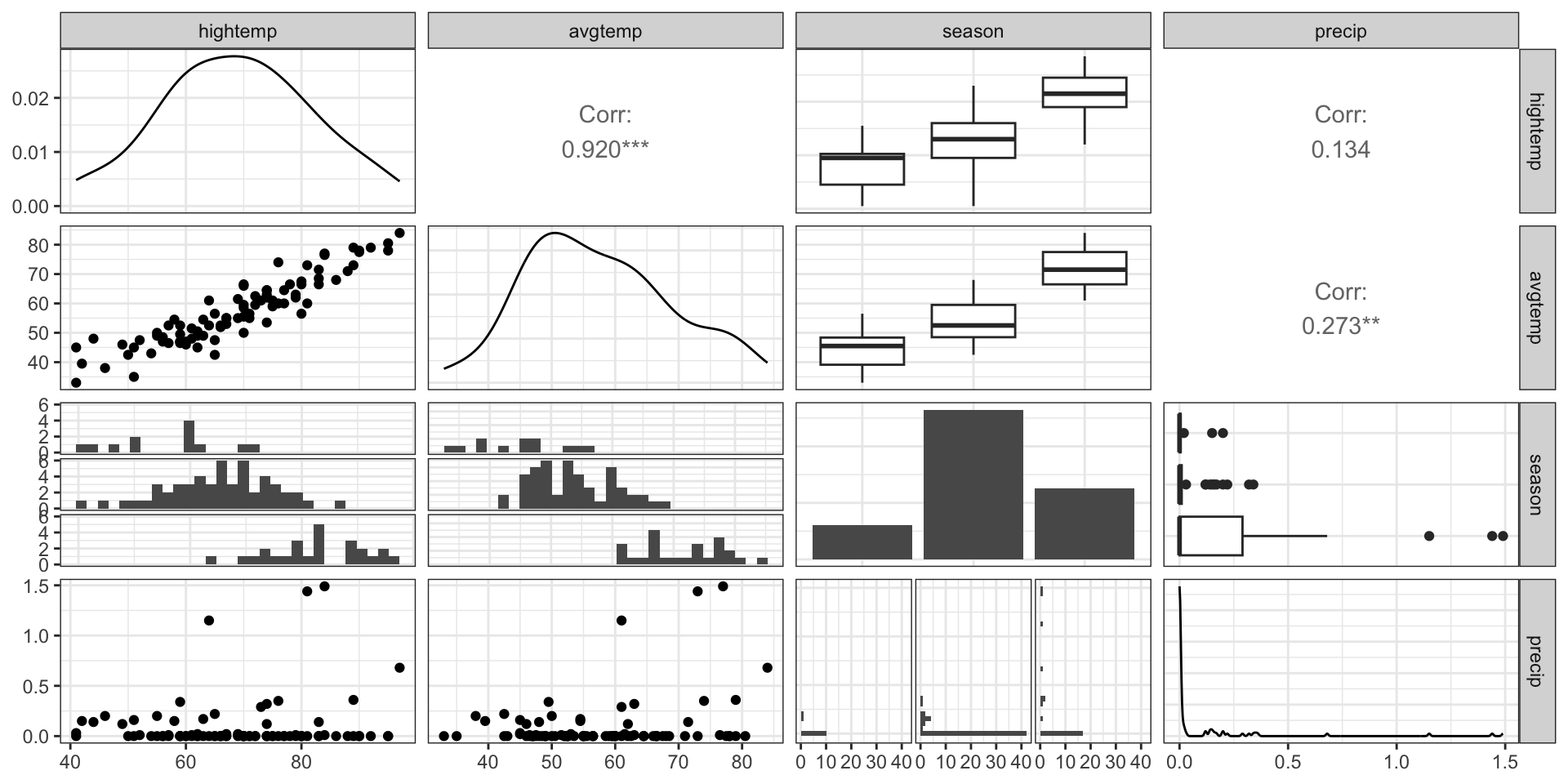
We can create a pairwise plot matrix using the ggpairs function from the GGally R package

rail_trail |>
  select(hightemp, avgtemp, season, precip) |>
  ggpairs()

EDA: Relationship between predictors

EDA: Correlation matrix

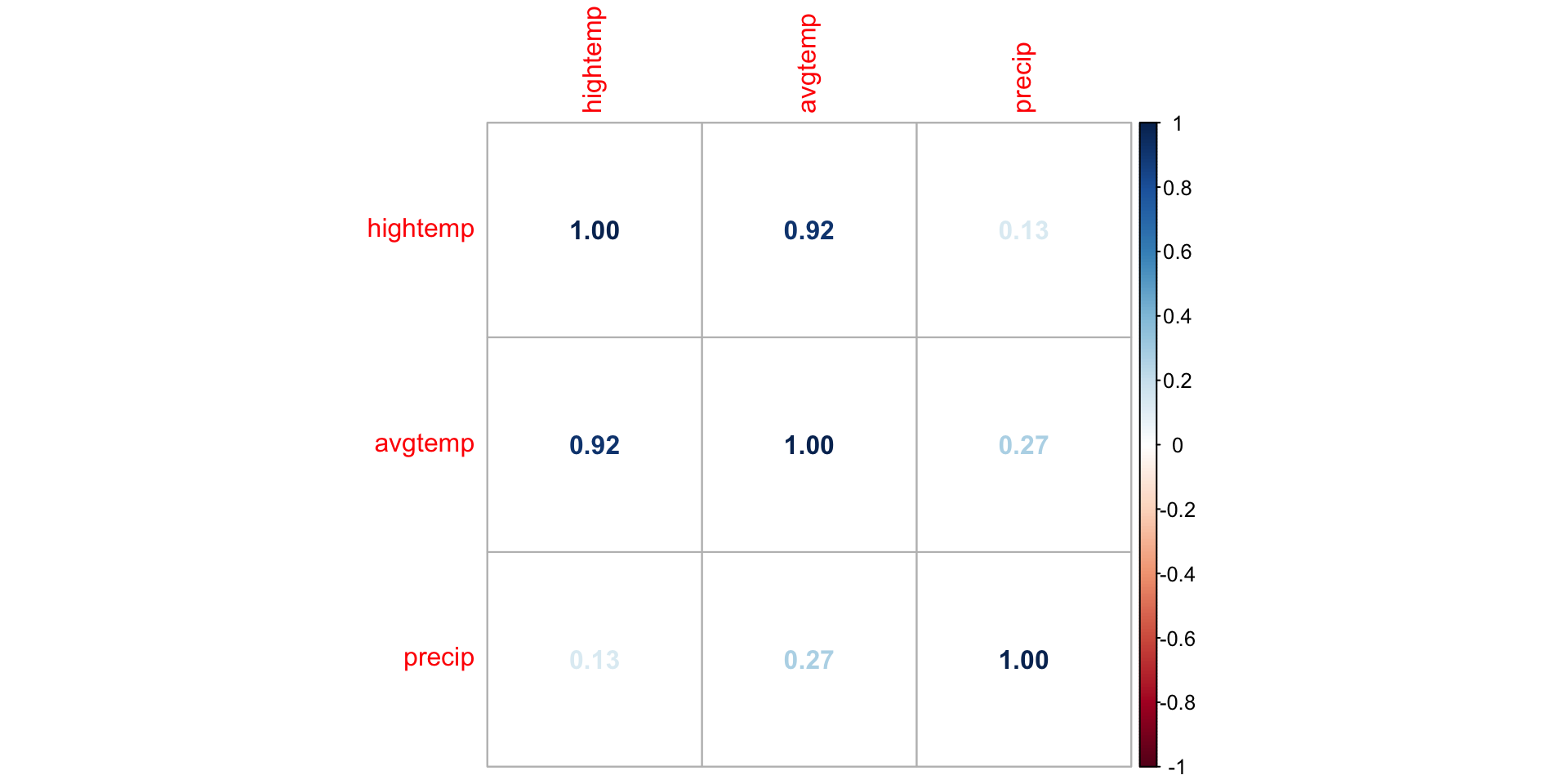
We can. use corrplot() in the corrplot R package to make a matrix of pairwise correlations between quantitative predictors

correlations <- rail_trail |>
  select(hightemp, avgtemp, precip) |>
  cor()

corrplot(correlations, method = "number")

EDA: Correlation matrix

What might be a potential concern with a model that uses high temperature, average temperature, season, and precipitation to predict volume?

Multicollinearity

Ideally the predictors are orthogonal, meaning they are completely independent of one another
In practice, there is typically some dependence between predictors but it is often not a major issue in the model
If there is linear dependence among (a subset of) the predictors, we cannot find estimate $\hat{β}$
If there are near-linear dependencies, we can find $\hat{β}$ but there may be other issues with the model
Multicollinearity: near-linear dependence among predictors

Sources of multicollinearity

Data collection method - only sample from a subspace of the region of predictors
Constraints in the population - e.g., predictors family income and size of house
Choice of model - e.g., adding high order terms to the model
Overdefined model - have more predictors than observations

Source: Montgomery, Peck, and Vining (2021)

Detecting multicollinearity

Recall $V a r (\hat{β}) = σ_{ϵ}^{2} (X^{T} X)^{- 1}$
Let $C = (X^{T} X)^{- 1}$ . Then $V a r ({\hat{β}}_{j}) = σ_{ϵ}^{2} C_{j j}$
When there are near-linear dependencies, $C_{j j}$ increases and thus $V a r ({\hat{β}}_{j})$ becomes inflated
$C_{j j}$ is associated with how much $V a r ({\hat{β}}_{j})$ is inflated due to $x_{j}$ dependencies with other predictors

Variance inflation factor

The variance inflation factor (VIF) measures how much the linear dependencies impact the variance of the predictors

$V I F_{j} = \frac{1}{1 - R_{j}^{2}}$

where $R_{j}^{2}$ is the proportion of variation in $x_{j}$ that is explained by a linear combination of all the other predictors

. . .

When the response and predictors are scaled in a particular way, $C_{j j} = V I F_{j}$ . Click here to see how.

Detecting multicollinearity

Common practice uses threshold $V I F > 10$ as indication of concerning multicollinearity (some say VIF > 5 is worth investigation)
Variables with similar values of VIF are typically the ones correlated with each other
Use the vif() function in the rms R package to calculate VIF

library(rms)

trail_fit <- lm(volume ~ hightemp + avgtemp + precip, data = rail_trail)

vif(trail_fit)

hightemp  avgtemp   precip 
7.161882 7.597154 1.193431

How multicollinearity impacts model

Large variance for the model coefficients that are collinear
- Different combinations of coefficient estimates produce equally good model fits
Unreliable statistical inference results
- May conclude coefficients are not statistically significant when there is, in fact, a relationship between the predictors and response
Interpretation of coefficient is no longer “holding all other variables constant”, since this would be impossible for correlated predictors

Application exercise

📋 sta221-sp25.netlify.app/ae/ae-04-multicollinearity.html

Part 1

Dealing with multicollinearity

Collect more data (often not feasible given practical constraints)
Redefine the correlated predictors to keep the information from predictors but eliminate collinearity
- e.g., if $x_{1}, x_{2}, x_{3}$ are correlated, use a new variable $(x_{1} + x_{2}) / x_{3}$ in the model
For categorical predictors, avoid using levels with very few observations as the baseline
Remove one of the correlated variables
- Be careful about substantially reducing predictive power of the model

Application exercise

📋 sta221-sp25.netlify.app/ae/ae-04-multicollinearity.html

Part 2

Recap

Introduced multicollinearity
- Definition
- How it impacts the model
- How to detect it
- What to do about it

References

Montgomery, Douglas C, Elizabeth A Peck, and G Geoffrey Vining. 2021. Introduction to Linear Regression Analysis. John Wiley & Sons.