# load packages
library(tidyverse)
library(tidymodels)
library(knitr)
library(patchwork)
library(GGally)   # for pairwise plot matrix
library(corrplot) # for correlation matrix

# set default theme in ggplot2
ggplot2::theme_set(ggplot2::theme_bw())Multicollinearity cont’d
Announcements
Exam corrections (optional) due TODAY at 11:59pm
Team Feedback (email from TEAMMATES) due TODAY at 11:59pm (check email)
Next project milestone: Exploratory data analysis due March 20
- Work on it in lab March 7
DataFest: April 4 - 6 - https://dukestatsci.github.io/datafest/
Computing set up
Topics
Multicollinearity
Recap
How to deal with issues of multicollinearity
Data: Trail users
- The Pioneer Valley Planning Commission (PVPC) collected data at the beginning a trail in Florence, MA for ninety days from April 5, 2005 to November 15, 2005.
- Data collectors set up a laser sensor, with breaks in the laser beam recording when a rail-trail user passed the data collection station.
# A tibble: 5 × 7
  volume hightemp avgtemp season cloudcover precip day_type
   <dbl>    <dbl>   <dbl> <chr>       <dbl>  <dbl> <chr>
1    501       83    66.5 Summer       7.60  0     Weekday
2    419       73    61   Summer       6.30  0.290 Weekday
3    397       74    63   Spring       7.5   0.320 Weekday
4    385       95    78   Summer       2.60  0     Weekend
5    200       44    48   Spring      10     0.140 Weekday
Source: Pioneer Valley Planning Commission via the mosaicData package.
Variables
Outcome:
volumeestimated number of trail users that day (number of breaks recorded)
Predictors
hightempdaily high temperature (in degrees Fahrenheit)avgtempaverage of daily low and daily high temperature (in degrees Fahrenheit)seasonone of “Fall”, “Spring”, or “Summer”precipmeasure of precipitation (in inches)
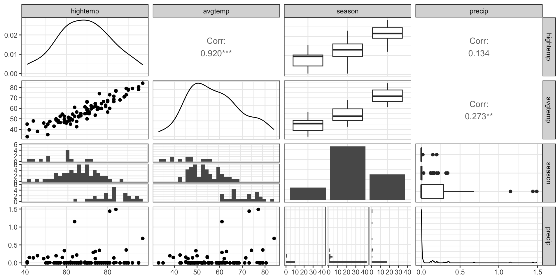
EDA: Relationship between predictors
Multicollinearity
Multicollinearity: near-linear dependence among predictors
The variance inflation factor (VIF) measures how much the linear dependencies impact the variance of the predictors
\[ VIF_{j} = \frac{1}{1 - R^2_j} \]
where \(R^2_j\) is the proportion of variation in \(x_j\) that is explained by a linear combination of all the other predictors
- Thresholds:
- VIF > 10: concerning multicollinearity
- VIF > 5: potentially worth further investigation
How multicollinearity impacts model
Large variance for the model coefficients that are collinear
- Different combinations of coefficient estimates produce equally good model fits
Unreliable statistical inference results
- May conclude coefficients are not statistically significant when there is, in fact, a relationship between the predictors and response
Interpretation of coefficient is no longer “holding all other variables constant”, since this would be impossible for correlated predictors
Dealing with multicollinearity
Collect more data (often not feasible given practical constraints)
Redefine the correlated predictors to keep the information from predictors but eliminate collinearity
- e.g., if \(x_1, x_2, x_3\) are correlated, use a new variable \((x_1 + x_2) / x_3\) in the model
For categorical predictors, avoid using levels with very few observations as the baseline
Remove one of the correlated variables
- Be careful about substantially reducing predictive power of the model