Logistic Regression: Prediction

Author

Prof. Maria Tackett

Published

Apr 01, 2025

Announcements

Next project milestone: Analysis and draft in April 11 lab
Team Feedback (email from TEAMMATES) due Tuesday, April 8 at 11:59pm (check email)
Statistics experience due April 22

Computational set up

library(tidyverse)
library(tidymodels)
library(pROC)       # make ROC curves
library(knitr)
library(kableExtra)

# set default theme in ggplot2
ggplot2::theme_set(ggplot2::theme_bw())

Topics

Calculating predicted probabilities from the logistic regression model
Using predicted probabilities to classify observations
Make decisions and assess model performance using
- Confusion matrix
- ROC curve

Data: Risk of coronary heart disease

This data set is from an ongoing cardiovascular study on residents of the town of Framingham, Massachusetts. We want to examine the relationship between various health characteristics and the risk of having heart disease.

high_risk: 1 = High risk of having heart disease in next 10 years, 0 = Not high risk of having heart disease in next 10 years
age: Age at exam time (in years)
totChol: Total cholesterol (in mg/dL)
currentSmoker: 0 = nonsmoker; 1 = smoker

Modeling risk of coronary heart disease

term	estimate	std.error	statistic	p.value	conf.low	conf.high
(Intercept)	-6.638	0.372	-17.860	0.000	-7.374	-5.917
age	0.082	0.006	14.430	0.000	0.071	0.093
totChol	0.002	0.001	2.001	0.045	0.000	0.004
currentSmoker1	0.457	0.092	4.951	0.000	0.277	0.639

Interpret totChol in terms of the odds of being high risk for heart disease.
Interpret currentSmoker1 in terms of the odds of being high risk for heart disease.

Prediction and classification

We are often interested in using the model to classify observations, i.e., predict whether a given observation will have a 1 or 0 response
For each observation
- Use the logistic regression model to calculate the predicted log-odds the response for the $i^{t h}$ observation is 1
- Use the log-odds to calculate the predicted probability the $i^{t h}$ observation is 1
- Then, use the predicted probability to classify the observation as having a 1 or 0 response using some predefined threshold

Augmented data frame

augment(heart_disease_fit)

# A tibble: 4,190 × 10
   high_risk   age totChol currentSmoker .fitted .resid     .hat .sigma  .cooksd
   <fct>     <dbl>   <dbl> <fct>           <dbl>  <dbl>    <dbl>  <dbl>    <dbl>
 1 0            39     195 0              -3.06  -0.302 0.000594  0.890  6.94e-6
 2 0            46     250 0              -2.38  -0.420 0.000543  0.890  1.25e-5
 3 0            48     245 1              -1.77  -0.560 0.000527  0.890  2.24e-5
 4 1            61     225 1              -0.751  1.51  0.00164   0.889  8.70e-4
 5 0            46     285 1              -1.86  -0.539 0.000830  0.890  3.25e-5
 6 0            43     228 0              -2.67  -0.366 0.000546  0.890  9.43e-6
 7 1            63     205 0              -1.08   1.66  0.00154   0.889  1.15e-3
 8 0            45     313 1              -1.88  -0.532 0.00127   0.890  4.86e-5
 9 0            52     260 0              -1.87  -0.535 0.000542  0.890  2.08e-5
10 0            43     225 1              -2.22  -0.454 0.000532  0.890  1.44e-5
# ℹ 4,180 more rows
# ℹ 1 more variable: .std.resid <dbl>

Predicted log-odds

heart_disease_aug <- augment(heart_disease_fit)

# A tibble: 5 × 1
  .fitted
    <dbl>
1  -3.06 
2  -2.38 
3  -1.77 
4  -0.751
5  -1.86

. . .

Observation 1

$predicted log-odds = \log (\frac{\hat{π}}{1 - \hat{π}}) = - 3.06$

Predicted odds

# A tibble: 5 × 1
  .fitted
    <dbl>
1  -3.06 
2  -2.38 
3  -1.77 
4  -0.751
5  -1.86

. . .

Observation 1

$predicted odds = \frac{\hat{π}}{1 - \hat{π}} = \exp {- 3.06} = 0.0469$

Predicted probability

# A tibble: 5 × 1
  .fitted
    <dbl>
1  -3.06 
2  -2.38 
3  -1.77 
4  -0.751
5  -1.86

. . .

Observation 1

$predicted prob. = \hat{π} = \frac{\hat{odds}}{1 + \hat{odds}} = \frac{\exp {- 3.06}}{1 + \exp {- 3.06}} = 0.045$

. . .

Would you classify this individual as high risk $(\hat{y} = 1)$ or not high risk $(\hat{y} = 0)$ ?

Another individual

# A tibble: 5 × 1
  .fitted
    <dbl>
1  -3.06 
2  -2.38 
3  -1.77 
4  -0.751
5  -1.86

. . .

Observation 4

$predicted prob. = \hat{π} = \frac{\hat{odds}}{1 + \hat{odds}} = \frac{\exp {- 0.751}}{1 + \exp {- 0.751}} = 0.321$

. . .

Would you classify this individual as high risk $(\hat{y} = 1)$ or not high risk $(\hat{y} = 0)$ ?

Predicted probabilities in R

We can calculate predicted probabilities using the predict.glm() function. Use type = "response" to get probabilities.¹

. . .

predict.glm(heart_disease_fit, type = "response")

. . .

Predicted probabilities for Observations 1 -5

         1          2          3          4          5 
0.04459439 0.08445209 0.14523257 0.32065849 0.13515474

Predictions in R

pred_prob <- predict.glm(heart_disease_fit, type = "response")

heart_disease_aug <- heart_disease_aug |> 
  bind_cols(pred_prob = pred_prob)

. . .

# A tibble: 5 × 3
  high_risk .fitted pred_prob
  <fct>       <dbl>     <dbl>
1 0          -3.06     0.0446
2 0          -2.38     0.0845
3 0          -1.77     0.145 
4 1          -0.751    0.321 
5 0          -1.86     0.135

Classifying observations

You would like to determine a threshold for classifying individuals as high risk or not high risk.

What considerations would you make in determining the threshold?

Classify using 0.5 as threshold

We can use a threshold of 0.5 to classify observations.

If $\hat{π} > 0.5$ , classify as 1
If $\hat{π} \leq 0.5$ , classify as 0

. . .

# A tibble: 5 × 4
  high_risk .fitted pred_prob pred_class
  <fct>       <dbl>     <dbl> <fct>     
1 0          -3.06     0.0446 0         
2 0          -2.38     0.0845 0         
3 0          -1.77     0.145  0         
4 1          -0.751    0.321  0         
5 0          -1.86     0.135  0

Confusion matrix

A confusion matrix is a $2 \times 2$ table that compares the predicted and actual classes. We can produce this matrix using the conf_mat() function in the yardstick package (part of tidymodels).

. . .

heart_disease_aug |>
  conf_mat(high_risk, pred_class)

          Truth
Prediction    0    1
         0 3553  635
         1    2    0

Visualize confusion matrix

heart_conf_mat <- heart_disease_aug |>
  conf_mat(high_risk, pred_class)

autoplot(heart_conf_mat, type = "heatmap")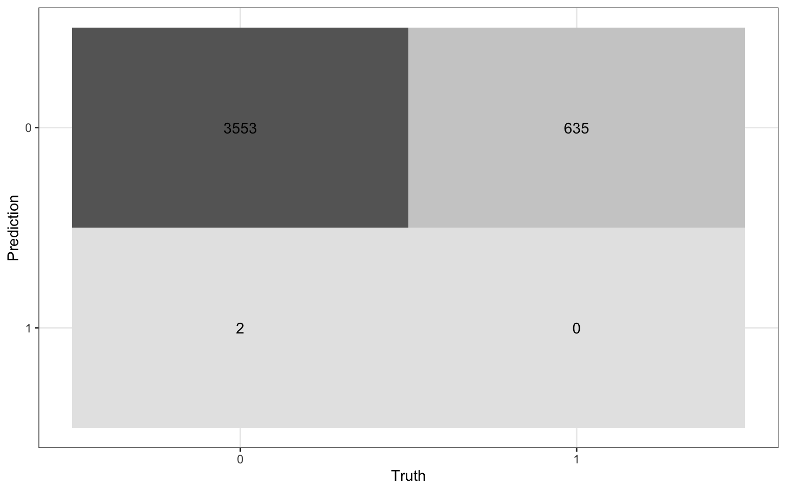

Using the confusion matrix

          Truth
Prediction    0    1
         0 3553  635
         1    2    0

. . .

The accuracy of this model with a classification threshold of 0.5 is

$accuracy = \frac{3553 + 0}{3553 + 635 + 2 + 0} = 0.848$

Using the confusion matrix

          Truth
Prediction    0    1
         0 3553  635
         1    2    0

. . .

The misclassification rate of this model with a threshold of 0.5 is

$misclassification = \frac{635 + 2}{3553 + 635 + 2 + 0} = 0.152$

Using the confusion matrix

          Truth
Prediction    0    1
         0 3553  635
         1    2    0

Accuracy is 0.848 and the misclassification rate is 0.152.

. . .

What is the limitation of solely relying on accuracy and misclassification to assess the model performance?
What is the limitation of using a single confusion matrix to assess the model performance?

Sensitivity and specificity

True/false positive/negative

	Not high risk $(y_{i} = 0)$	High risk $(y_{i} = 1)$
Classified not high risk $({\hat{π}}_{i} \leq threshold)$	True negative (TN)	False negative (FN)
Classified high risk $({\hat{π}}_{i} > threshold)$	False positive (FP)	True positive (TP)

$accuracy = \frac{T N + T P}{T N + T P + F N + F P}$
$misclassification = \frac{F N + F P}{T N + T P + F N + F P}$

False negative rate

	Not high risk $(y_{i} = 0)$	High risk $(y_{i} = 1)$
Classified not high risk $({\hat{π}}_{i} \leq threshold)$	True negative (TN)	False negative (FN)
Classified high risk $({\hat{π}}_{i} > threshold)$	False positive (FP)	True positive (TP)

. . .

False negative rate: Proportion of actual positives that were classified as negatives

P(classified not high risk | high risk) = $\frac{F N}{T P + F N}$

False positive rate

	Not high risk $(y_{i} = 0)$	High risk $(y_{i} = 1)$
Classified not high risk $({\hat{π}}_{i} \leq threshold)$	True negative (TN)	False negative (FN)
Classified high risk $({\hat{π}}_{i} > threshold)$	False positive (FP)	True positive (TP)

. . .

False positive rate: Proportion of actual negatives that were classified as positives

P(classified high risk | not high risk) = $\frac{F P}{T N + F P}$

Sensitivity

	Not high risk $(y_{i} = 0)$	High risk $(y_{i} = 1)$
Classified not high risk $({\hat{π}}_{i} \leq threshold)$	True negative (TN)	False negative (FN)
Classified high risk $({\hat{π}}_{i} > threshold)$	False positive (FP)	True positive (TP)

. . .

Sensitivity: Proportion of actual positives that were correctly classified as positive

Also known as true positive rate (TPR) and recall
P(classified high risk | high risk) = 1 − False negative rate

Specificity

	Not high risk $(y_{i} = 0)$	High risk $(y_{i} = 1)$
Classified not high risk $({\hat{π}}_{i} \leq threshold)$	True negative (TN)	False negative (FN)
Classified high risk $({\hat{π}}_{i} > threshold)$	False positive (FP)	True positive (TP)

. . .

Specificity: Proportion of actual negatives that were correctly classified as negative

P(classified not high risk | not high risk) = 1 − False positive rate

Practice

          Truth
Prediction    0    1
         0 3553  635
         1    2    0

Calculate the

False negative rate
False positive rate
Sensitivity
Specificity

Using metrics to select model and threshold

Metric	Guidance for use
Accuracy	For balanced data, use only in combination with other metrics. Avoid using for imbalanced data.
Sensitivity (true positive rate)	Use when false negatives are more “expensive” than false positives.
False positive rate	Use when false positives are more “expensive” than false negatives.
Precision = $\frac{T P}{T P + F P}$	Use when it’s important for positive predictions to be accurate.

This table is a modification of work created and shared by Google in the Google Machine Learning Crash Course.

Choosing a classification threshold

A doctor plans to use your model to determine which patients are high risk for heart disease. The doctor will recommend a treatment plan for high risk patients.

Would you want sensitivity to be high or low? What about specificity?
What are the trade-offs associated with each decision?

ROC curve

So far the model assessment has depended on the model and selected threshold. The receiver operating characteristic (ROC) curve allows us to assess the model performance across a range of thresholds.

. . .

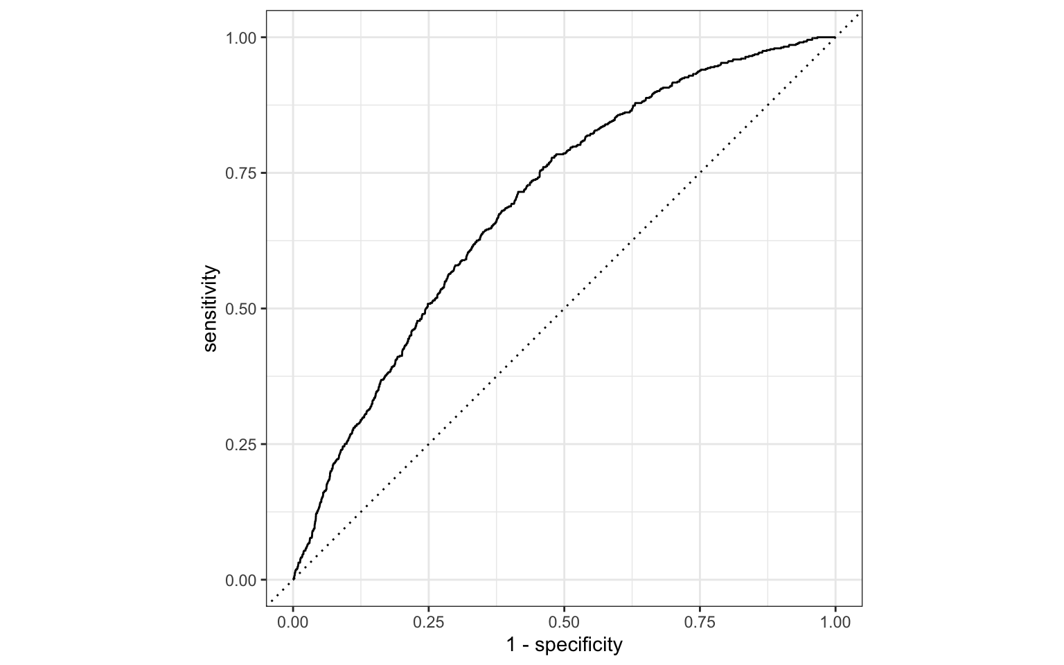
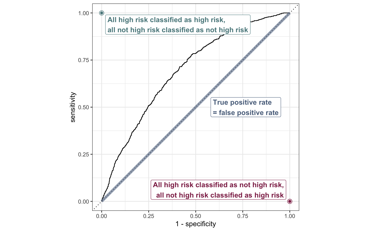
x-axis: 1 - Specificity (False positive rate)
y-axis: Sensitivity (True positive rate)

Which corner of the plot indicates the best model performance?

ROC curve

ROC curve in R

# calculate sensitivity and specificity at each threshold
roc_curve_data <- heart_disease_aug |>
  roc_curve(high_risk, pred_prob, 
            event_level = "second") 

# plot roc curve
autoplot(roc_curve_data)

ROC curve in R

Sample from underlying data

# A tibble: 10 × 3
   .threshold specificity sensitivity
        <dbl>       <dbl>       <dbl>
 1     0.0545       0.103       0.980
 2     0.0660       0.181       0.959
 3     0.0832       0.305       0.909
 4     0.136        0.583       0.715
 5     0.193        0.754       0.501
 6     0.221        0.805       0.411
 7     0.221        0.805       0.411
 8     0.262        0.881       0.287
 9     0.270        0.901       0.254
10     0.279        0.915       0.227

Area under the curve

The area under the curve (AUC) can be used to assess how well the logistic model fits the data

AUC=0.5: model is a very bad fit (no better than a coin flip)
AUC close to 1: model is a good fit

. . .

heart_disease_aug |>
  roc_auc(high_risk, pred_prob,
    event_level = "second"
  )

# A tibble: 1 × 3
  .metric .estimator .estimate
  <chr>   <chr>          <dbl>
1 roc_auc binary         0.695

Recap

Calculated predicted probabilities from the logistic regression model
Used predicted probabilities to classify observations
Made decisions and assessed model performance using
- Confusion matrix
- ROC curve

Footnotes

The default is type = "link", which produces the predicted log-odds.↩︎

Announcements

Computational set up

Topics

Data: Risk of coronary heart disease

Modeling risk of coronary heart disease

Prediction and classification

Augmented data frame

Predicted log-odds

Predicted odds

Predicted probability

Another individual

Predicted probabilities in R

Predictions in R

Classifying observations

Classify using 0.5 as threshold

Confusion matrix

Visualize confusion matrix

Using the confusion matrix

Using the confusion matrix

Using the confusion matrix

Sensitivity and specificity

True/false positive/negative

False negative rate

False positive rate

Sensitivity

Specificity

Practice

Using metrics to select model and threshold

Choosing a classification threshold

ROC curve

ROC curve

ROC curve in R

ROC curve in R

Area under the curve

Recap

Further reading

Footnotes