Probabilities, odds, odds ratios

Author

Prof. Maria Tackett

Published

Mar 24, 2025

Announcements

Project Presentations in lab on Friday, March 28
Lab 06 due TODAY at 11:59pm
Statistics experience due April 22

Drop-in Peer Advising will be happening Wednesday, March 26, from 6:30-8:30 PM in Bostock Lounge for students to stop by with any questions they have around STA/CS/MATH classes, major pathways, or other general advice since shopping carts just opened.

Fall 2025 STA classes

STA 240: Probability for Statistical Inference, Modeling, and Data Analysis (or STA 230 or STA 231)
STA 322: Study Design: Design of Surveys and Causal Studies
STA 323: Statistical Computing
STA 325: Machine Learning and Data Mining (need STA 230/231/240)
STA 332: Statistical Inference (need STA 230/231/240)
STA 344: Introduction to Statistical Modeling of Spatial and Time Series data (need STA 230/231/240)
STA 402: Bayesian Statistical Modeling and Data Analysis (need STA 332)
STA 465: Introduction to High Dimensional Data Analysis

Topics

Review: Multicollinearity vs. interaction effects
Logistic regression for binary response variable
Relationship between odds and probabilities
Odds ratios

Computational setup

# load packages
library(tidyverse)
library(tidymodels)
library(knitr)
library(patchwork)
library(Stat2Data) #contains sleep data set

# set default theme in ggplot2
ggplot2::theme_set(ggplot2::theme_bw())

Review: Multicollinearity vs. interactions

Suppose we fit a model using flipper length and bill length to understand variability in body mass for Palmer Penguins. We make the plots below as part of the EDA.

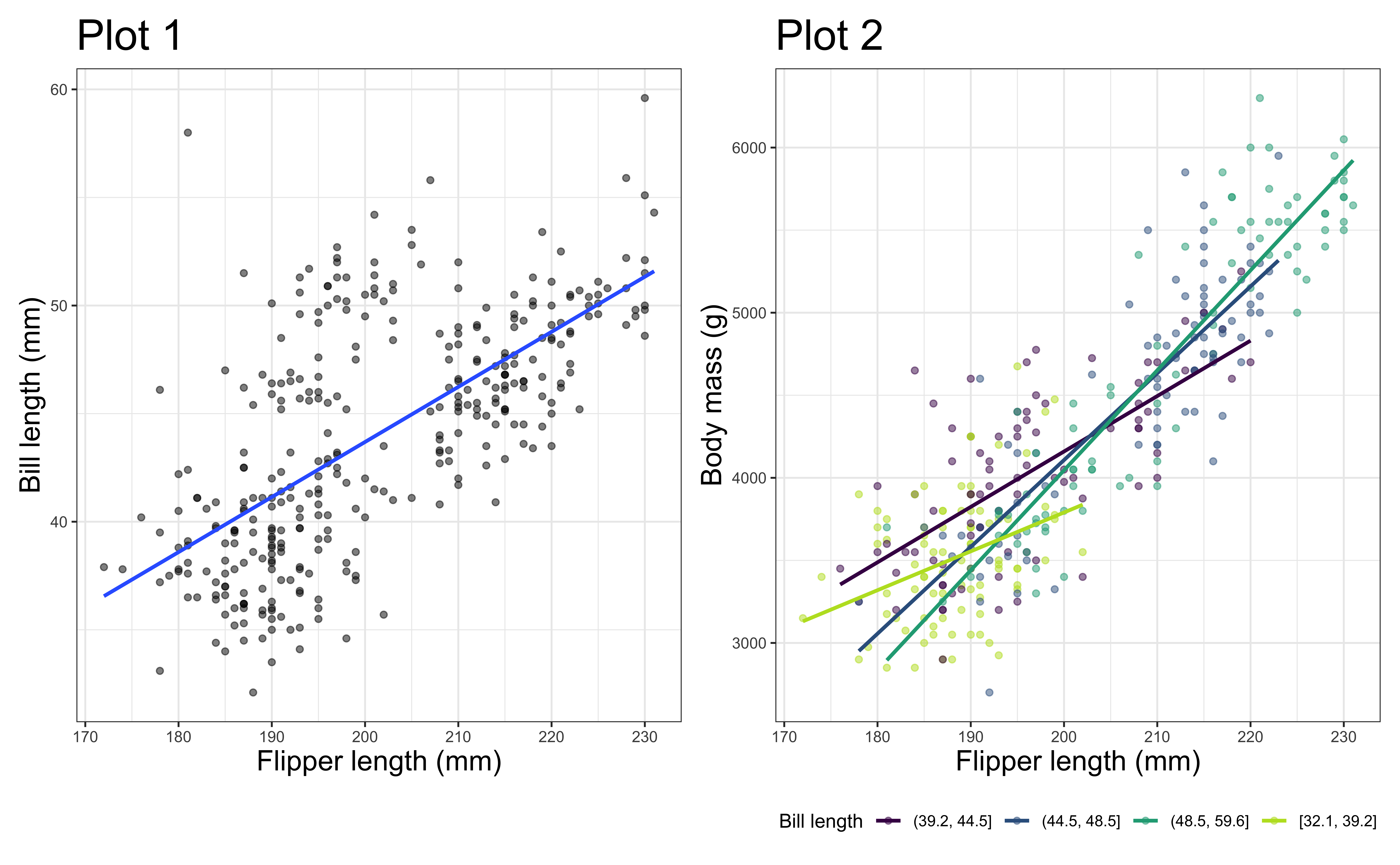
What are we checking in Plot 1? In Plot 2?

Predicting categorical outcomes

Types of outcome variables

Quantitative outcome variable:

Sales price of a house in Duke Forest
Model: Expected sales price given the number of bedrooms, lot size, etc.

. . .

Categorical outcome variable:

Indicator of being high risk of getting coronary heart disease in the next 10 years
Model: Probability an adult is high risk of heart disease in the next 10 years given their age, total cholesterol, etc.

Models for categorical outcomes

Logistic regression

2 Outcomes

1: Yes, 0: No

Multinomial logistic regression

3+ Outcomes

1: Democrat, 2: Republican, 3: Independent

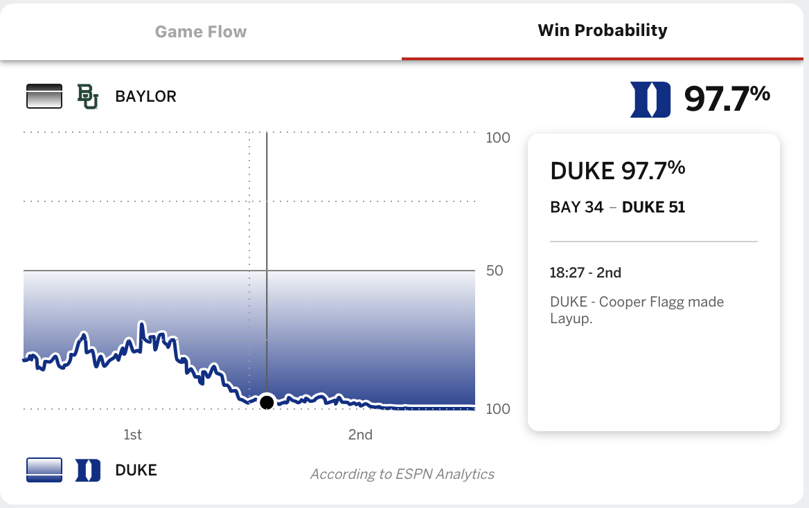
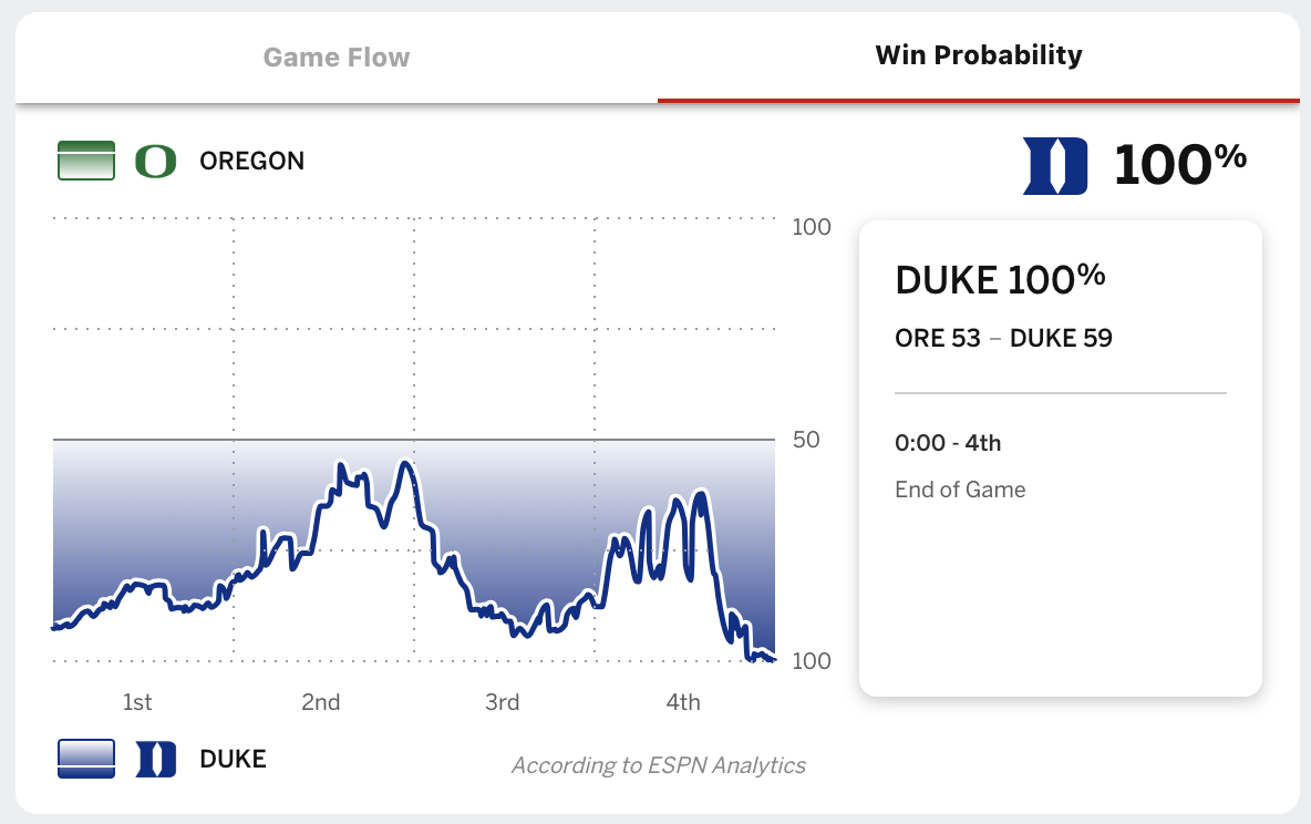
Example: Win probabilities

Duke in 2nd round of NCCA March Madness Tournaments

Men’s Basketball

Women’s Basketball

Do teenagers get 7+ hours of sleep?

Students in grades 9 - 12 were surveyed about health risk behaviors including whether they usually get 7 or more hours of sleep.

Sleep7

1: yes

0: no

# A tibble: 446 × 2
     Age Sleep7
   <int>  <int>
 1    16      1
 2    17      0
 3    18      0
 4    17      1
 5    15      0
 6    17      0
 7    17      1
 8    16      1
 9    16      1
10    18      0
# ℹ 436 more rows

Plot the data

ggplot(sleep, aes(x = Age, y = Sleep7)) +
  geom_point() + 
  labs(y = "Getting 7+ hours of sleep")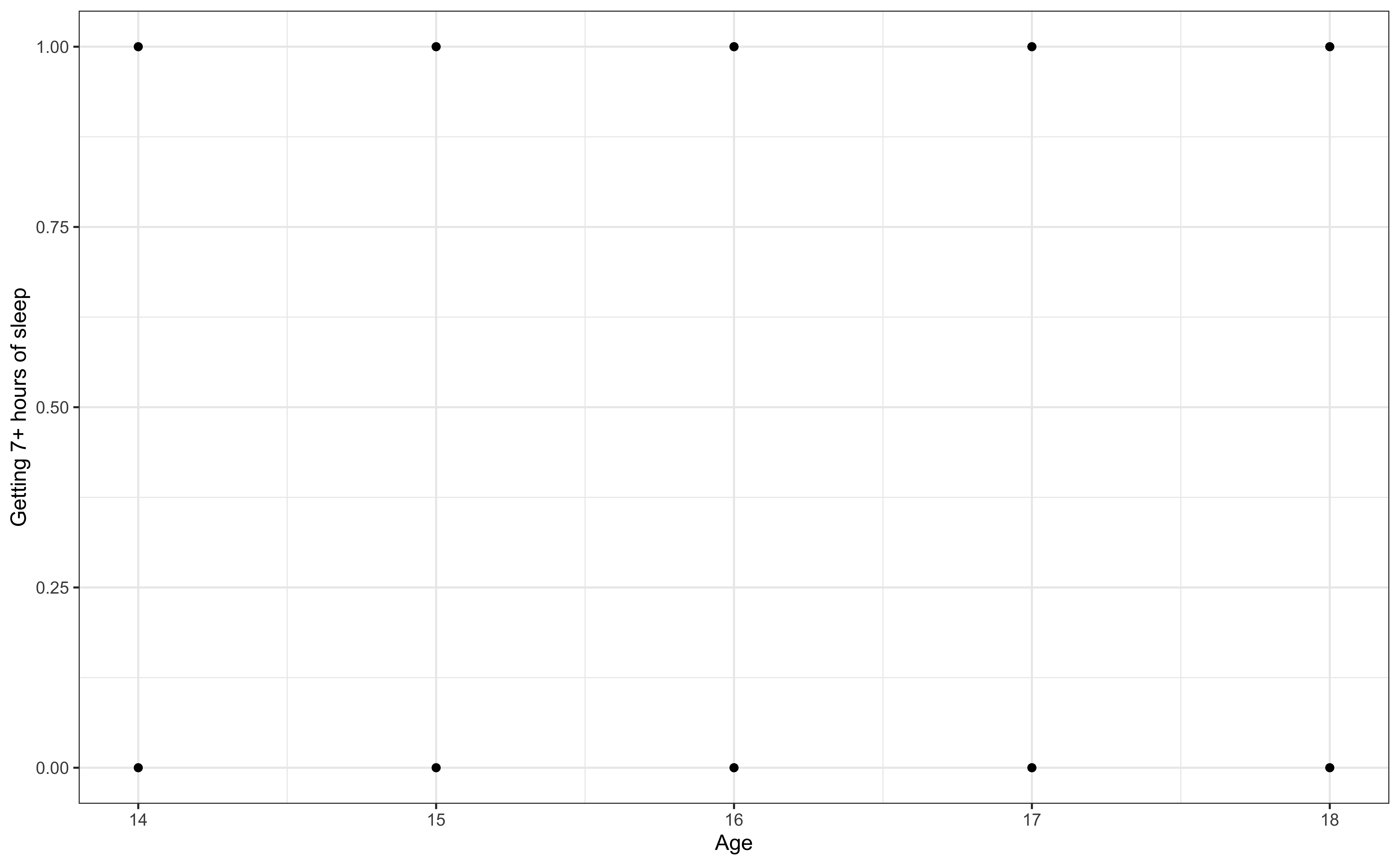

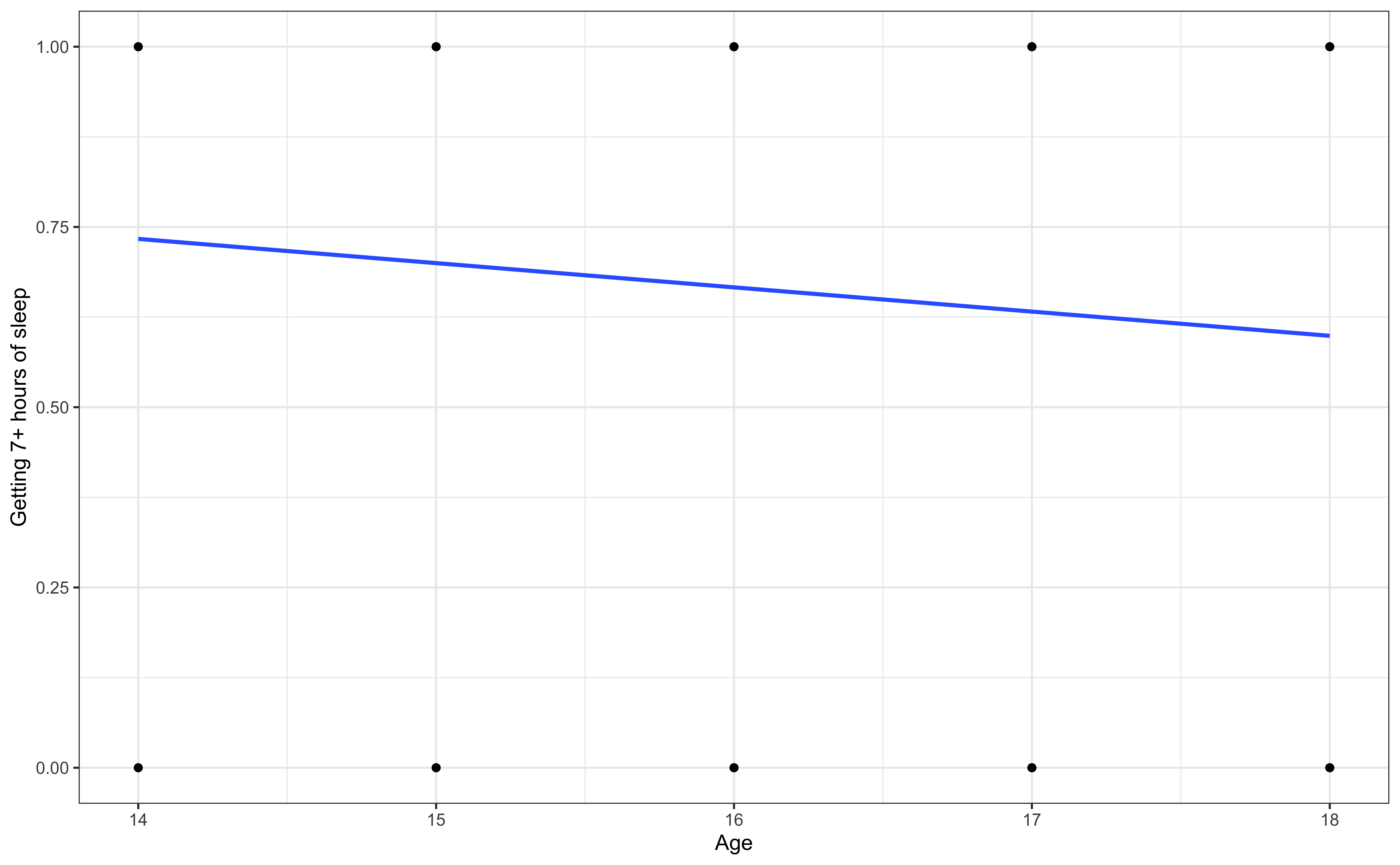
Let’s fit a linear regression model

Outcome: $Y$ = 1: yes, 0: no

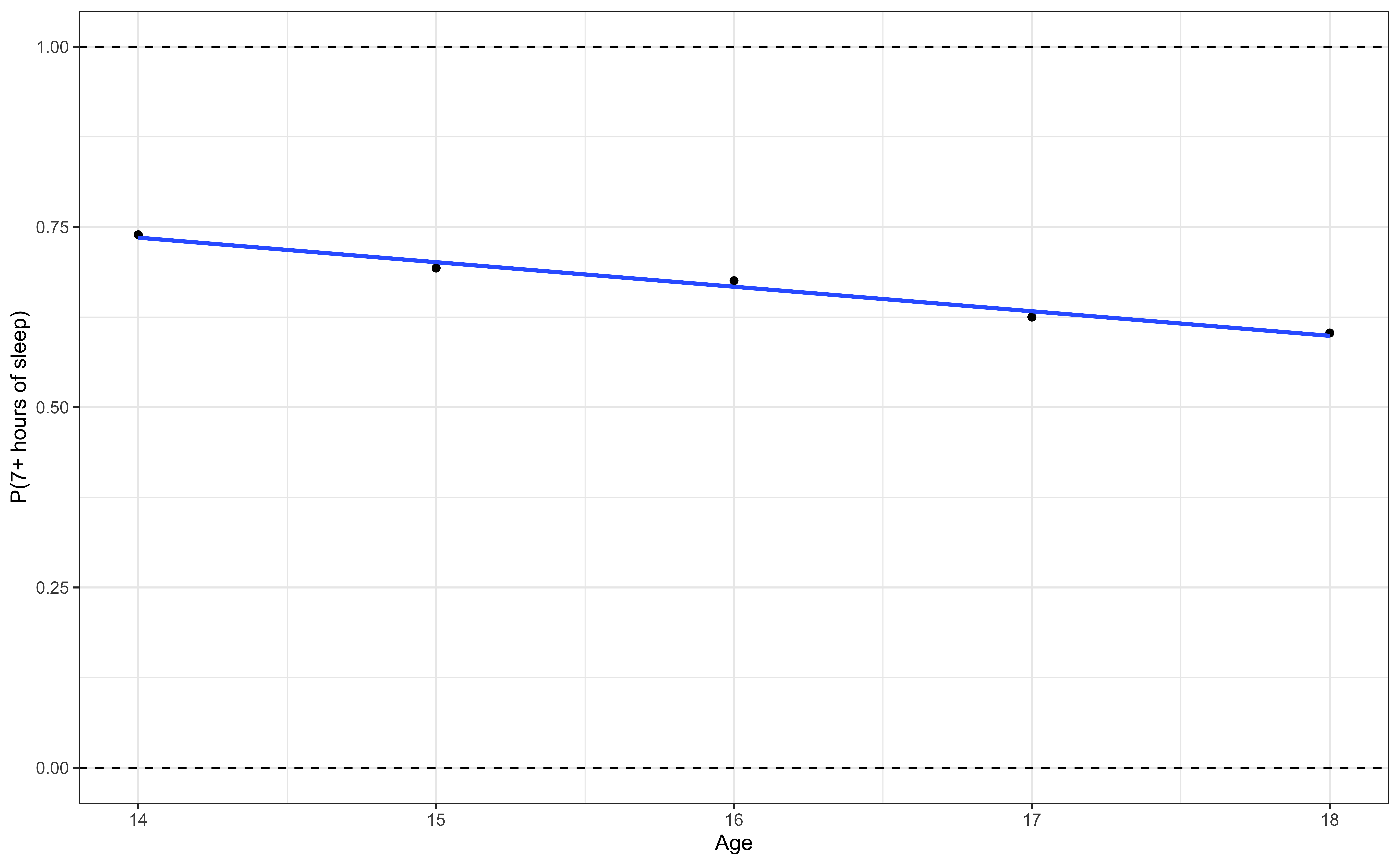
Let’s use proportions

Outcome: Probability of getting 7+ hours of sleep

What happens if we zoom out?

Outcome: Probability of getting 7+ hours of sleep

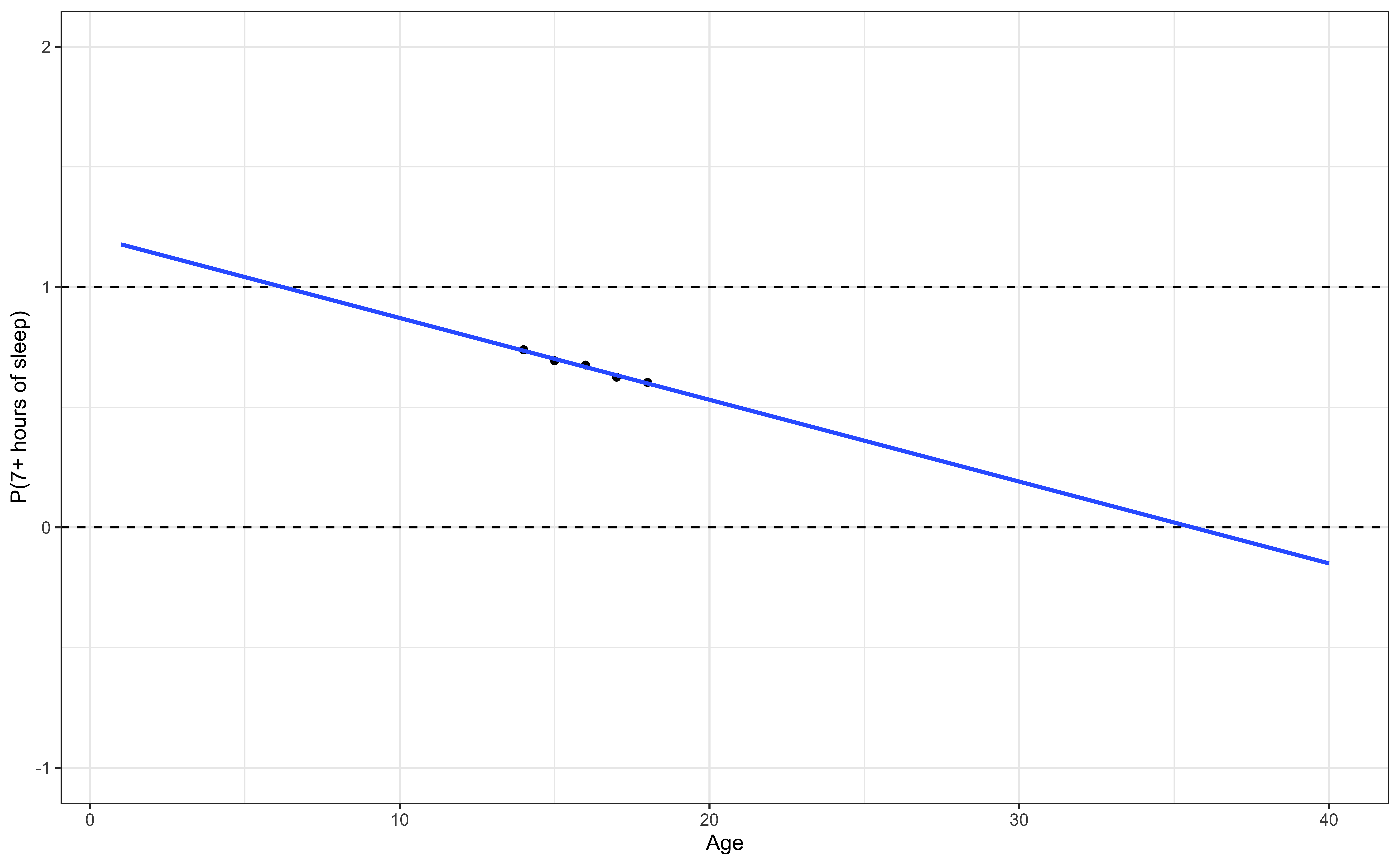
🛑 This model produces predictions outside of 0 and 1.

Let’s try another model

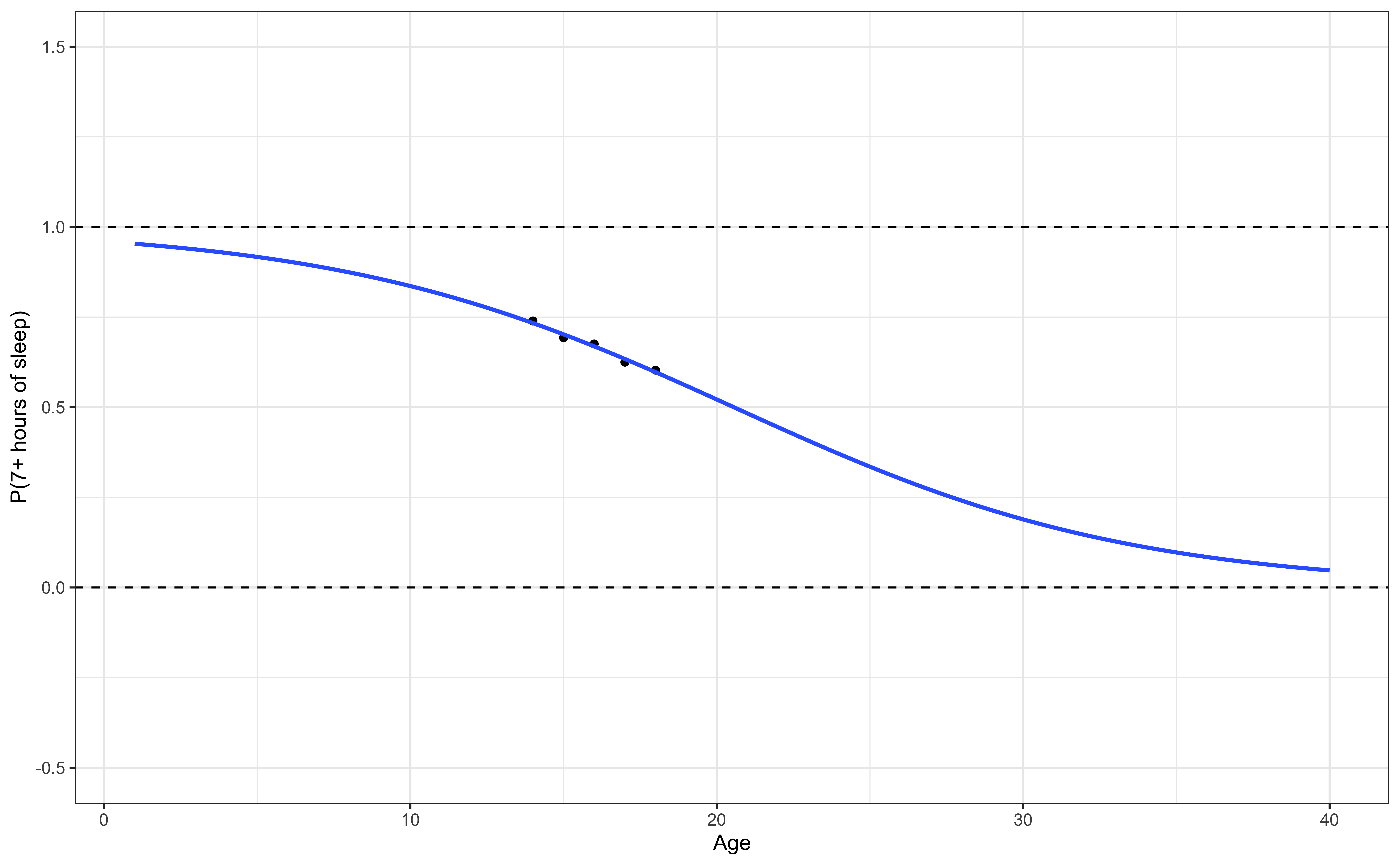
✅ This model (called a logistic regression model) only produces predictions between 0 and 1.

The code

ggplot(sleep_age, aes(x = Age, y = prop)) +
  geom_point() + 
  geom_hline(yintercept = c(0,1), lty = 2) + 
  stat_smooth(method ="glm", method.args = list(family = "binomial"), 
              fullrange = TRUE, se = FALSE) +
  labs(y = "P(7+ hours of sleep)") +
  xlim(1, 40) +
  ylim(-0.5, 1.5)

Different types of models

Method	Outcome	Model
Linear regression	Quantitative	$y = X β + ϵ$
Linear regression (transform Y)	Quantitative	$\log (y) = X β + ϵ$
Logistic regression	Binary	$\log (\frac{π}{1 - π}) = X β$

Linear vs. logistic regression

State whether a linear regression model or logistic regression model is more appropriate for each scenario.

Use age and political party to predict if a randomly selected person will vote in the next election.
Use budget and run time (in minutes) to predict a movie’s total revenue.
Use age and sex to calculate the probability a randomly selected adult will visit Duke Health in the next year.

Probabilities and odds

Data: Concern about rising AI

This data comes from the 2023 Pew Research Center’s American Trends Panel. The survey aims to capture public opinion about a variety of topics including politics, religion, and technology, among others. We will use data from 11201 respondents in Wave 132 of the survey conducted July 31 - August 6, 2023.

The goal of this analysis is to understand the relationship between age, how much someone has heard about artificial intelligence (AI), and concern about the increased use of AI in daily life.

A more complete analysis on this topic can be found in the Pew Research Center article Growing public concern about the role of artificial intelligence in daily life by Alec Tyson and Emma Kikuchi.

Variables

ai_concern: Whether a respondent said they are “more concerned than excited” about in the increased use of AI in daily life (1: yes, 0: no)

Variables

ai_heard : Response to the question “How much have you heard or read about AI?”
- A lot
- A little
- Nothing at all
- Refused
age_cat: Age category
- 18-29
- 30-49
- 50-64
- 65+
- Refused

Data prep

# change variable names and recode categories
pew_data <- pew_data |>
  mutate(ai_concern = if_else(CNCEXC_W132 == 2, 1, 0),
         age_cat = case_when(F_AGECAT == 1 ~ "18-29",
                             F_AGECAT == 2 ~ "30-49",
                             F_AGECAT == 3 ~ "50-64",
                             F_AGECAT == 4 ~ "65+",
                             TRUE ~ "Refused"), 
         ai_heard = case_when(AI_HEARD_W132 == 1 ~ "A lot",
                              AI_HEARD_W132 == 2 ~ "A little",
                              AI_HEARD_W132 == 3 ~ "Nothing at all",
                              TRUE ~ "Refused"
                              ))

# Make factors and  relevel 
pew_data <- pew_data |>
  mutate(ai_concern = factor(ai_concern),
         age_cat = factor(age_cat), 
         ai_heard = factor(ai_heard, levels = c("A lot", "A little", "Nothing at all", "Refused"))
  )

Univariate EDA

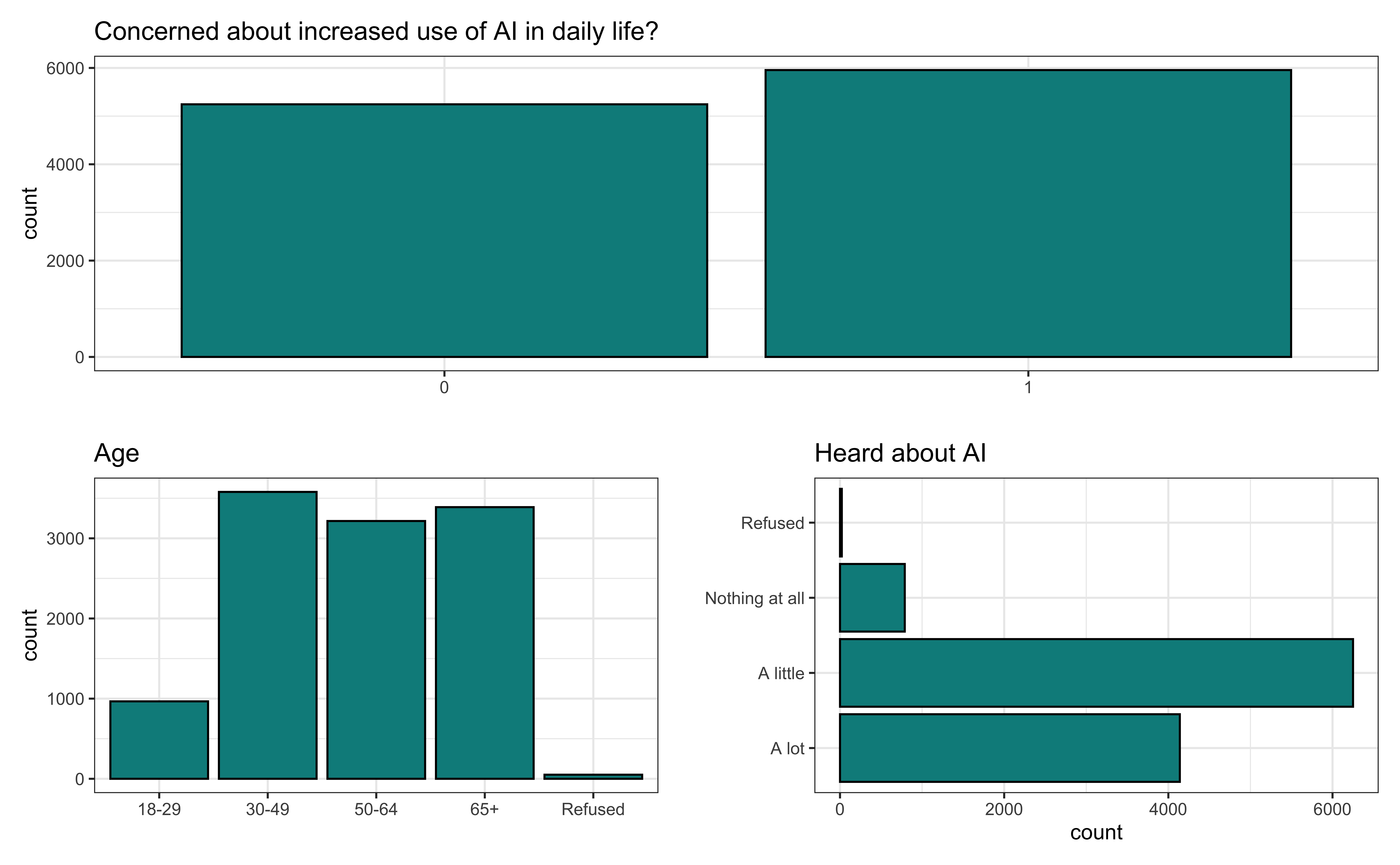
Binary response variable

$Y = 1 : yes (success), 0 : no (failure)$
$π$ : probability that $Y = 1$ , i.e., $P (Y = 1)$
$\frac{π}{1 - π}$ : odds that $Y = 1$
$\log (\frac{π}{1 - π})$ : log odds
Go from $π$ to $\log (\frac{π}{1 - π})$ using the logit transformation

Example

Suppose there is a 70% chance it will rain tomorrow

Probability it will rain is $π = 0.7$
Probability it won’t rain is $1 - π = 0.3$
Odds it will rain are 7 to 3, 7:3, $\frac{0.7}{0.3} \approx 2.33$

Concerned about AI in daily life?

pew_data |>
  count(ai_concern) |>
  mutate(pi = round(n / sum(n), 3))

# A tibble: 2 × 3
  ai_concern     n    pi
  <fct>      <int> <dbl>
1 0           5245 0.468
2 1           5956 0.532

. . .

$P (Concerned about AI) = P (Y = 1) = π = 0.532$

. . .

$P (Not concerned about AI) = P (Y = 0) = 1 - π = 0.468$

. . .

$Odds of being concerned about AI = \frac{0.532}{0.468} = 1.137$

From odds to probabilities

odds

$odds = \frac{π}{1 - π}$

probability

$π = \frac{odds}{1 + odds}$

Odds ratios

Concern about AI vs. age

Age	Not Concerned	Concerned
18-29	550	416
30-49	1898	1681
50-64	1398	1818
65+	1376	2013
Refused	23	28

Compare the odds for two groups

Age	Not Concerned	Concerned
18-29	550	416
30-49	1898	1681
50-64	1398	1818
65+	1376	2013
Refused	23	28

. . .

We want to compare concern about increased use of AI in daily life between individuals who are 18-29 years old to those who are 65+ years old

Compare the odds for two groups

Age	Not Concerned	Concerned
18-29	550	416
30-49	1898	1681
50-64	1398	1818
65+	1376	2013
Refused	23	28

We’ll use the odds to compare the two groups

$odds = \frac{P (success)}{P (failure)} = \frac{# of successes}{# of failures}$

Compare the odds for two groups

Age	Not Concerned	Concerned
18-29	550	416
30-49	1898	1681
50-64	1398	1818
65+	1376	2013
Refused	23	28

Odds of being concerned with increased use of AI in daily life for 18-29 year olds: $\frac{416}{550} = 0.756$
Odds of being concerned with increased use of AI in daily life for those who are 65+ years old: $\frac{2013}{1376} = 1.463$
Based on this, we see that individuals 65+ years old are more likely to be concerned about the increased use of AI in daily life than 18-29 year olds.

Odds ratio (OR)

Age	Not Concerned	Concerned
18-29	550	416
30-49	1898	1681
50-64	1398	1818
65+	1376	2013
Refused	23	28

Let’s summarize the relationship between the two groups. To do so, we’ll use the odds ratio (OR).

$O R = \frac{{odds}_{1}}{{odds}_{2}}$

OR: AI concern by age

Age	Not Concerned	Concerned
18-29	550	416
30-49	1898	1681
50-64	1398	1818
65+	1376	2013
Refused	23	28

$O R = \frac{{odds}_{18 - 29}}{{odds}_{65 +}} = \frac{0.756}{1.463} = 0.517$

. . .

The odds an 18-29 year old is concerned about increased use of AI in daily life are 0.517 times the odds a 65+ year old is concerned.

More natural interpretation

It’s more natural to interpret the odds ratio with a statement with the odds ratio greater than 1.
The odds a 65+ year old is concerned about increased use of AI in daily life are 1.934 (1/0.517) times the odds an 18-29 year old is concerned.

Code to make table

pew_data |>
  count(age_cat, ai_concern)

# A tibble: 10 × 3
   age_cat ai_concern     n
   <fct>   <fct>      <int>
 1 18-29   0            550
 2 18-29   1            416
 3 30-49   0           1898
 4 30-49   1           1681
 5 50-64   0           1398
 6 50-64   1           1818
 7 65+     0           1376
 8 65+     1           2013
 9 Refused 0             23
10 Refused 1             28

Code to make table

pew_data |>
  count(age_cat, ai_concern) |>
  pivot_wider(names_from = ai_concern, values_from = n)

# A tibble: 5 × 3
  age_cat   `0`   `1`
  <fct>   <int> <int>
1 18-29     550   416
2 30-49    1898  1681
3 50-64    1398  1818
4 65+      1376  2013
5 Refused    23    28

Code to make table

pew_data |>
  count(age_cat, ai_concern) |>
  pivot_wider(names_from = ai_concern, values_from = n) |>
  kable()

age_cat	0	1
18-29	550	416
30-49	1898	1681
50-64	1398	1818
65+	1376	2013
Refused	23	28

Code to make table

pew_data |>
  count(age_cat, ai_concern) |>
  pivot_wider(names_from = ai_concern, values_from = n) |>
  kable(col.names = c("Age", "Not concerned", "Concerned"))

Age	Not concerned	Concerned
18-29	550	416
30-49	1898	1681
50-64	1398	1818
65+	1376	2013
Refused	23	28

Application exercise

📋 sta221-sp25.netlify.app/ae/ae-05-prob-odds.html

Recap

Introduced logistic regression for binary response variable
Showed the relationship between odds and probabilities
Introduced odds ratios